10.2 Implementing “Simple” Subprograms |
443 |
10.2 Implementing “Simple” Subprograms
We begin with the task of implementing simple subprograms. By “simple” we mean that subprograms cannot be nested and all local variables are static. Early versions of Fortran were examples of languages that had this kind of subprograms.
The semantics of a call to a “simple” subprogram requires the following actions:
1.Save the execution status of the current program unit.
2.Compute and pass the parameters.
3.Pass the return address to the called.
4.Transfer control to the called.
The semantics of a return from a simple subprogram requires the following actions:
1.If there are pass-by-value-result or out-mode parameters, the current values of those parameters are moved to or made available to the corresponding actual parameters.
2.If the subprogram is a function, the functional value is moved to a place accessible to the caller.
3.The execution status of the caller is restored.
4.Control is transferred back to the caller.
The call and return actions require storage for the following:
•Status information about the caller
•Parameters
•Return address
•Return value for functions
•Temporaries used by the code of the subprograms
These, along with the local variables and the subprogram code, form the complete collection of information a subprogram needs to execute and then return control to the caller.
The question now is the distribution of the call and return actions to the caller and the called. For simple subprograms, the answer is obvious for most of the parts of the process. The last three actions of a call clearly must be done by the caller. Saving the execution status of the caller could be done by either. In the case of the return, the first, third, and fourth actions must be done by the called. Once again, the restoration of the execution status of the caller could be done by either the caller or the called. In general, the linkage actions of the called can occur at two different times, either at the beginning of its execution or at the end. These are sometimes called the prologue and epilogue of the subprogram linkage. In the case of a simple subprogram, all of the linkage actions of the callee occur at the end of its execution, so there is no need for a prologue.

444 |
Chapter 10 Implementing Subprograms |
A simple subprogram consists of two separate parts: the actual code of the subprogram, which is constant, and the local variables and data listed previously, which can change when the subprogram is executed. In the case of simple subprograms, both of these parts have fixed sizes.
The format, or layout, of the noncode part of a subprogram is called an activation record, because the data it describes are relevant only during the activation, or execution of the subprogram. The form of an activation record is static. An activation record instance is a concrete example of an activation record, a collection of data in the form of an activation record.
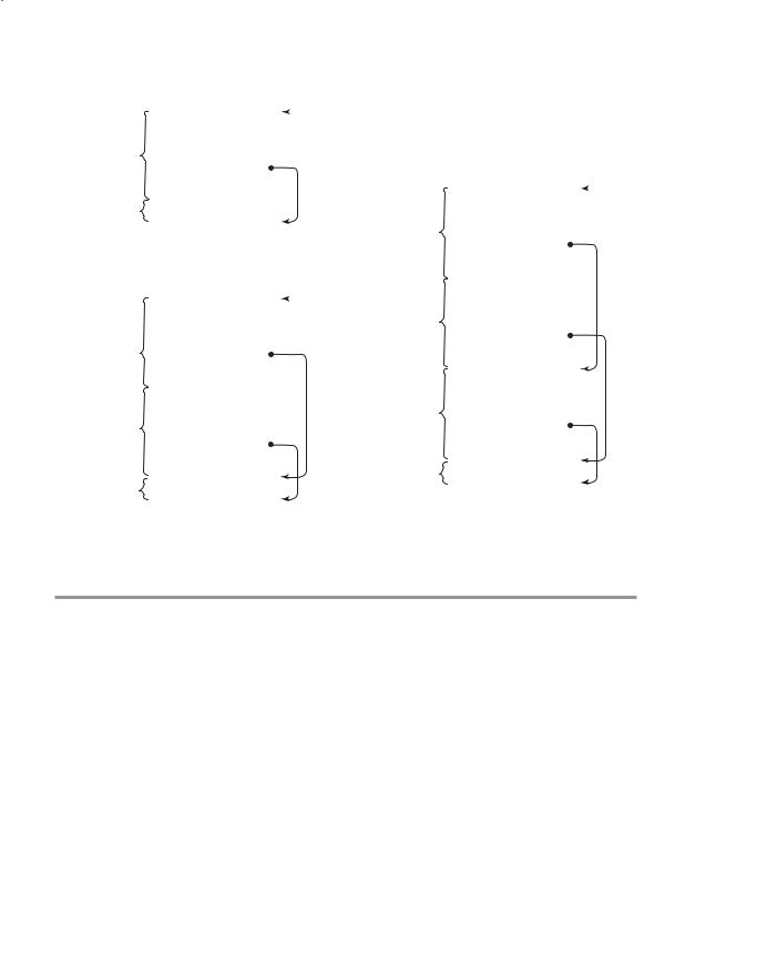
Because languages with simple subprograms do not support recursion, there can be only one active version of a given subprogram at a time. Therefore, there can be only a single instance of the activation record for a subprogram. One possible layout for activation records is shown in Figure 10.1. The saved execution status of the caller is omitted here and in the remainder of this chapter because it is simple and not relevant to the discussion.
Figure 10.1 |
|
Local variables |
|
|
|
|
|
An activation record for |
|
|
|
|
Parameters |
|
|
simple subprograms |
|
|
|
|
|
|
|
|
Return address |
|
|
|
|
|
|
|
|
|
|
|
|
Because an activation record instance for a “simple” subprogram has fixed |
|
|
size, it can be statically allocated. In fact, it could be attached to the code part |
||
|
of the subprogram. |
||
|
|
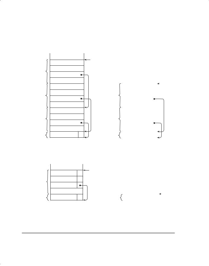
Figure 10.2 shows a program consisting of a main program and three |
|
|
subprograms: A, B, and C. Although the figure shows all the code segments |
||
|
separated from all the activation record instances, in some cases, the activation |
||
|
record instances are attached to their associated code segments. |
||
|
|
The construction of the complete program shown in Figure 10.2 is not done |
|
|
entirely by the compiler. In fact, if the language allows independent compilation, |
||
|
the four program units—MAIN, A, B, and C—may have been compiled on different |
||
|
days, or even in different years. At the time each unit is compiled, the machine |
||
|
code for it, along with a list of references to external subprograms, is written to a |
||
|
file. The executable program shown in Figure 10.2 is put together by the linker, |
||
|
which is part of the operating system. (Sometimes linkers are called loaders, linker/ |
||
|
loaders, or link editors.) When the linker is called for a main program, its first task |
||
|
is to find the files that contain the translated subprograms referenced in that pro- |
||
|
gram and load them into memory. Then, the linker must set the target addresses |
||
|
of all calls to those subprograms in the main program to the entry addresses of |
||
|
those subprograms. The same must be done for all calls to subprograms in the |
||
|
loaded subprograms and all calls to library subprograms. In the previous example, |
||
|
the linker was called for MAIN. The linker had to find the machine code programs |
||
|
for A, B, and C, along with their activation record instances, and load them into |
||
|
10.3 Implementing Subprograms with Stack-Dynamic Local Variables |
445 |
|
Figure 10.2 |
MAIN |
Local variables |
|
|
|
||
The code and |
|
Local variables |
|
|
|
|
|
activation records of |
A |
Parameters |
|
a program with simple |
|
Return address |
|
subprograms |
Data |
|
|
Local variables |
|
||
|
|
|
|
|
B |
Parameters |
|
|
|
Return address |
|
|
|
Local variables |
|
|
C |
Parameters |
|
Return address
MAIN
A
Code
B
C
memory with the code for MAIN. Then, it had to patch in the target addresses for all calls to A, B, C, and any library subprograms in A, B, C, and MAIN.
10.3Implementing Subprograms with Stack-Dynamic Local Variables
We now examine the implementation of the subprogram linkage in languages in which locals are stack dynamic, again focusing on the call and return operations.
One of the most important advantages of stack-dynamic local variables is support for recursion. Therefore, languages that use stack-dynamic local variables also support recursion.
A discussion of the additional complexity required when subprograms can be nested is postponed until Section 10.4.
10.3.1More Complex Activation Records
Subprogram linkage in languages that use stack-dynamic local variables are more complex than the linkage of simple subprograms for the following reasons:
•The compiler must generate code to cause the implicit allocation and deallocation of local variables.

446Chapter 10 Implementing Subprograms
•Recursion adds the possibility of multiple simultaneous activations of a subprogram, which means that there can be more than one instance (incomplete execution) of a subprogram at a given time, with at least one call from outside the subprogram and one or more recursive calls. The number of activations is limited only by the memory size of the machine. Each activation requires its activation record instance.
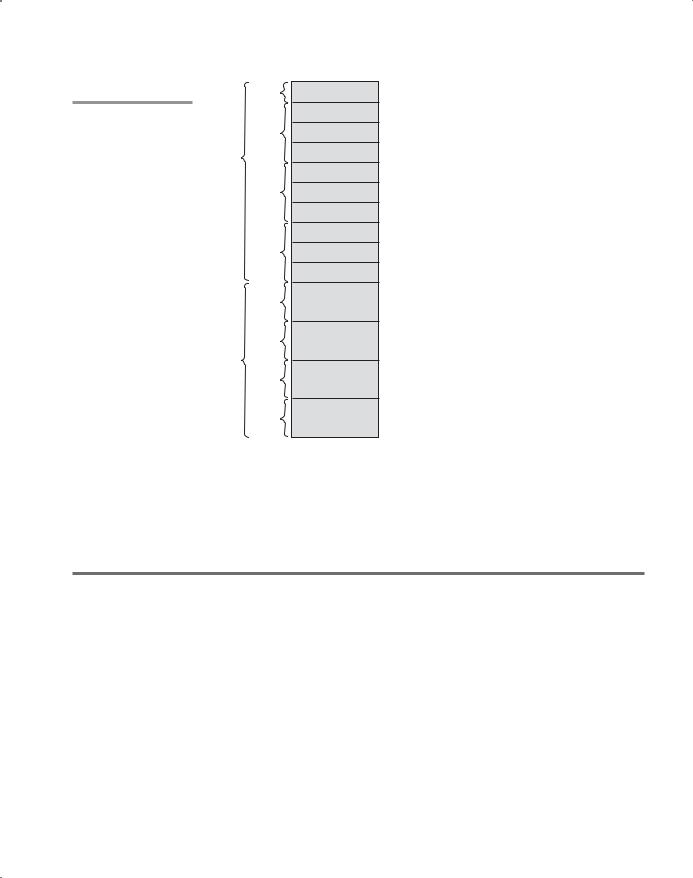
The format of an activation record for a given subprogram in most languages is known at compile time. In many cases, the size is also known for activation records because all local data are of a fixed size. That is not the case in some other languages, such as Ada, in which the size of a local array can depend on the value of an actual parameter. In those cases, the format is static, but the size can be dynamic. In languages with stack-dynamic local variables, activation record instances must be created dynamically. The typical activation record for such a language is shown in Figure 10.3.
Because the return address, dynamic link, and parameters are placed in the activation record instance by the caller, these entries must appear first.
Figure 10.3 |
|
Local variables |
|
|
A typical activation |
|
Parameters |
|
|
record for a language |
|
|
|
|
|
|
|
|
|
|
|
|
|
|
with stack-dynamic |
|
Dynamic link |
Stack top |
|
local variables |
|
|
|
|
|
Return address |
|
|
|
|
|
|
|
|
|
|
|
|
|
The return address usually consists of a pointer to the instruction following the call in the code segment of the calling program unit. The dynamic link is a pointer to the base of the activation record instance of the caller. In staticscoped languages, this link is used to provide traceback information when a run-time error occurs. In dynamic-scoped languages, the dynamic link is used to access nonlocal variables. The actual parameters in the activation record are the values or addresses provided by the caller.
Local scalar variables are bound to storage within an activation record instance. Local variables that are structures are sometimes allocated elsewhere, and only their descriptors and a pointer to that storage are part of the activation record. Local variables are allocated and possibly initialized in the called subprogram, so they appear last.
Consider the following skeletal C function:
void sub(float total, int part) {
int list[5];
float sum;
...
}
The activation record for sub is shown in Figure 10.4.
10.3 Implementing Subprograms with Stack-Dynamic Local Variables |
447 |
Figure 10.4
The activation record for function sub
Local |
sum |
|
list [4] |
Local |
|
|
list [3] |
Local |
|
|
list [2] |
Local |
|
|
list [1] |
Local |
|
|
list [0] |
Local |
|
|
part |
Parameter |
|
|
|
Parameter |
total |
|
|
Dynamic link |
|
|
|
Return address |
|
Activating a subprogram requires the dynamic creation of an instance of the activation record for the subprogram. As stated earlier, the format of the activation record is fixed at compile time, although its size may depend on the call in some languages. Because the call and return semantics specify that the subprogram last called is the first to complete, it is reasonable to create instances of these activation records on a stack. This stack is part of the runtime system and therefore is called the run-time stack, although we will usually just refer to it as the stack. Every subprogram activation, whether recursive or nonrecursive, creates a new instance of an activation record on the stack. This provides the required separate copies of the parameters, local variables, and return address.
One more thing is required to control the execution of a subprogram— the EP. Initially, the EP points at the base, or first address of the activation record instance of the main program. Therefore, the run-time system must ensure that it always points at the base of the activation record instance of the currently executing program unit. When a subprogram is called, the current EP is saved in the new activation record instance as the dynamic link. The EP is then set to point at the base of the new activation record instance. Upon return from the subprogram, the stack top is set to the value of the current EP minus one and the EP is set to the dynamic link from the activation record instance of the subprogram that has completed its execution. Resetting the stack top effectively removes the top activation record instance.

448 |
Chapter 10 Implementing Subprograms |
The EP is used as the base of the offset addressing of the data contents of the activation record instance—parameters and local variables.
Note that the EP currently being used is not stored in the run-time stack. Only saved versions are stored in the activation record instances as the dynamic links.
We have now discussed several new actions in the linkage process. The lists given in Section 10.2 must be revised to take these into account. Using the activation record form given in this section, the new actions are as follows:
The caller actions are as follows:
1.Create an activation record instance.
2.Save the execution status of the current program unit.
3.Compute and pass the parameters.
4.Pass the return address to the called.
5.Transfer control to the called.
The prologue actions of the called are as follows:
1.Save the old EP in the stack as the dynamic link and create the new value.
2.Allocate local variables.
The epilogue actions of the called are as follows:
1.If there are pass-by-value-result or out-mode parameters, the current values of those parameters are moved to the corresponding actual parameters.
2.If the subprogram is a function, the functional value is moved to a place accessible to the caller.
3.Restore the stack pointer by setting it to the value of the current EP minus one and set the EP to the old dynamic link.
4.Restore the execution status of the caller.
5.Transfer control back to the caller.
Recall from Chapter 9, that a subprogram is active from the time it is called until the time that execution is completed. At the time it becomes inactive, its local scope ceases to exist and its referencing environment is no longer meaningful. Therefore, at that time, its activation record instance can be destroyed.
Parameters are not always transferred in the stack. In many compilers for RISC machines, parameters are passed in registers. This is because RISC machines normally have many more registers than CISC machines. In the remainder of this chapter, however, we assume that parameters are passed in
10.3 Implementing Subprograms with Stack-Dynamic Local Variables |
449 |
the stack. It is straightforward to modify this approach for parameters being passed in registers.
10.3.2An Example Without Recursion
Consider the following skeletal C program:
void fun1(float r) { |
|
int s, t; |
1 |
... |
|
fun2(s); |
|
... |
|
} |
|
void fun2(int x) { |
|
int y; |
2 |
... |
|
fun3(y); |
|
... |
|
} |
|
void fun3(int q) { |
3 |
... |
|
} |
|
void main() { float p;
...
fun1(p);
...
}
The sequence of function calls in this program is
main calls fun1
fun1 calls fun2
fun2 calls fun3
The stack contents for the points labeled 1, 2, and 3 are shown in Figure 10.5.
At point 1, only the activation record instances for function main and function fun1 are on the stack. When fun1 calls fun2, an instance of fun2’s activation record is created on the stack. When fun2 calls fun3, an instance of fun3’s activation record is created on the stack. When fun3’s execution ends, the instance of its activation record is removed from the stack, and the EP is used to reset the stack top pointer. Similar processes take place when
450 |
Chapter 10 Implementing Subprograms |
|
|
|
|
|
|
|
|||||
|
|
|
|
|
|
|
|
|
|
|
|
Top |
|
|
|
|
|
|
|
|
|
|
|
|
|
||
|
|
|
|
|
|
|
|
|
Parameter |
|
|
||
|
|
|
|
|
|
|
|
ARI |
|
q |
|||
|
|
|
|
|
|
|
|
Dynamic link |
|
|
|
||
|
|
|
|
|
|
|
|
for fun3 |
|
|
|
||
|
|
|
|
|
|
|
|
|
|
|
|
||
|
|
|
|
|
|
|
|
Return (to fun2) |
|
|
|
||
|
|
|
|
|
|
|
|
|
|
|
|
||
|
|
|
|
|
|
|
|
|
|
|
|
||
|
|
|
|
|
|
|
|
|
|
|
|
|
|
|
|
|
|
|
|
|
|
Top |
Local |
|
y |
||
|
|
|
|
|
Local |
y |
|
||||||
|
|
|
|
|
|
|
|
||||||
|
|
|
|
ARI |
|
Parameter |
|
x |
|||||
|
|
|
|
Parameter |
x |
ARI |
|
||||||
|
|
|
|
|
|
||||||||
|
|
|
|
|
|
|
|
||||||
|
|
|
|
for fun2 |
|
|
|
Dynamic link |
|
|
|
||
|
|
|
|
Dynamic link |
|
|
|
|
|
||||
|
|
|
|
|
|
|
for fun2 |
|
|
|
|
||
|
|
|
|
|
|
|
Return (to fun1) |
|
|
|
|||
|
|
|
|
Top |
Return (to fun1) |
|
|
|
|
|
|
||
|
|
|
|
|
|
|
|
|
|
||||
|
|
|
|
|
|
|
|
|
|
|
|||
|
|
|
|
|
|
|
Local |
t |
|||||
|
|
|
|
|
|
|
|
||||||
|
Local |
|
t |
Local |
t |
|
|||||||
|
|
|
|
|
|||||||||
|
|
|
|
Local |
|||||||||
ARI |
Local |
|
s |
ARI |
Local |
s |
ARI |
s |
|||||
|
|
||||||||||||
|
Parameter |
||||||||||||
for fun1 |
Parameter |
|
|
Parameter |
|
|
r |
||||||
|
r for fun1 |
r for fun1 |
|||||||||||
|
|
||||||||||||
|
|
Dynamic link |
|
|
|
||||||||
|
Dynamic link |
|
|
|
Dynamic link |
|
|
|
|
|
|
||
|
|
|
|
|
|
|
|
|
|
|
|||
|
|
|
|
|
|
|
Return (to main) |
|
|
|
|||
|
Return (to main) |
|
|
|
Return (to main) |
|
|
|
|
|
|
||
|
|
|
ARI |
|
|
ARI |
|
|
|
|
|||
ARI |
|
p |
|
p |
Local |
p |
|||||||
Local |
Local |
||||||||||||
for main |
for main |
for main |
|||||||||||
at Point 1 |
|
|
at Point 2 |
|
|
at Point 3 |
|
|
|
||||
|
|
|
|
|
|
|
|
|
|
||||
ARI = activation record instance
Figure 10.5
Stack contents for three points in a program
functions fun2 and fun1 terminate. After the return from the call to fun1 from main, the stack has only the instance of the activation record of main. Note that some implementations do not actually use an activation record instance on the stack for main functions, such as the one shown in the figure. However, it can be done this way, and it simplifies both the implementation and our discussion. In this example and in all others in this chapter, we assume that the stack grows from lower addresses to higher addresses, although in a particular implementation, the stack may grow in the opposite direction.
The collection of dynamic links present in the stack at a given time is called the dynamic chain, or call chain. It represents the dynamic history of how execution got to its current position, which is always in the subprogram code whose activation record instance is on top of the stack. References to local variables can be represented in the code as offsets from the beginning of the activation record of the local scope, whose address is stored in the EP. Such an offset is called a local_offset.
The local_offset of a variable in an activation record can be determined at compile time, using the order, types, and sizes of variables declared in the subprogram associated with the activation record. To simplify the discussion,

10.3 Implementing Subprograms with Stack-Dynamic Local Variables |
451 |
we assume that all variables take one position in the activation record. The first local variable declared in a subprogram would be allocated in the activation record two positions plus the number of parameters from the bottom (the first two positions are for the return address and the dynamic link). The second local variable declared would be one position nearer the stack top and so forth. For example, consider the preceding example program. In fun1, the local_offset of s is 3; for t it is 4. Likewise, in fun2, the local_offset of y is 3. To get the address of any local variable, the local_offset of the variable is added to the EP.
10.3.3Recursion
Consider the following example C program, which uses recursion to compute the factorial function:
int factorial(int n) {
1
if (n <= 1)
return 1;
else return (n * factorial(n - 1));
2
}
void main() {
int value;
value = factorial(3);
3
}
The activation record format for the function factorial is shown in Figure 10.6. Notice that it has an additional entry for the return value of the function.
Figure 10.7 shows the contents of the stack for the three times execution reaches position 1 in the function factorial. Each shows one more activation of the function, with its functional value undefined. The first activation record instance has the return address to the calling function,
Figure 10.6 |
|
Functional value |
|
The activation record |
|
Parameter |
n |
for factorial |
|
||
|
|
|
|
|
Dynamic link |
|
|
|
|
|
|
|
|
|
|
|
|
Return address |
|
|
|
|
|