

3.5 Describing the Meanings of Programs: Dynamic Semantics |
139 |
grammars are a powerful and commonly used tool for compiler writers, who are more interested in the process of producing a compiler than they are in formalism.
3.5 Describing the Meanings of Programs: Dynamic Semantics
We now turn to the difficult task of describing the dynamic semantics, or meaning, of the expressions, statements, and program units of a programming language. Because of the power and naturalness of the available notation, describing syntax is a relatively simple matter. On the other hand, no universally accepted notation or approach has been devised for dynamic semantics. In this section, we briefly describe several of the methods that have been developed. For the remainder of this section, when we use the term semantics, we mean dynamic semantics.
There are several different reasons underlying the need for a methodology and notation for describing semantics. Programmers obviously need to know precisely what the statements of a language do before they can use them effectively in their programs. Compiler writers must know exactly what language constructs mean to design implementations for them correctly. If there were a precise semantics specification of a programming language, programs written in the language potentially could be proven correct without testing. Also, compilers could be shown to produce programs that exhibited exactly the behavior given in the language definition; that is, their correctness could be verified. A complete specification of the syntax and semantics of a programming language could be used by a tool to generate a compiler for the language automatically. Finally, language designers, who would develop the semantic descriptions of their languages, could in the process discover ambiguities and inconsistencies in their designs.
Software developers and compiler designers typically determine the semantics of programming languages by reading English explanations in language manuals. Because such explanations are often imprecise and incomplete, this approach is clearly unsatisfactory. Due to the lack of complete semantics specifications of programming languages, programs are rarely proven correct without testing, and commercial compilers are never generated automatically from language descriptions.
Scheme, a functional language described in Chapter 15, is one of only a few programming languages whose definition includes a formal semantics description. However, the method used is not one described in this chapter, as this chapter is focused on approaches that are suitable for imperative languages.
3.5.1 Operational Semantics
The idea behind operational semantics is to describe the meaning of a statement or program by specifying the effects of running it on a machine. The effects on the machine are viewed as the sequence of changes in its

140 |
Chapter 3 Describing Syntax and Semantics |
state, where the machine’s state is the collection of the values in its storage. An obvious operational semantics description, then, is given by executing a compiled version of the program on a computer. Most programmers have, on at least one occasion, written a small test program to determine the meaning of some programming language construct, often while learning the language. Essentially, what such a programmer is doing is using operational semantics to determine the meaning of the construct.
There are several problems with using this approach for complete formal semantics descriptions. First, the individual steps in the execution of machine language and the resulting changes to the state of the machine are too small and too numerous. Second, the storage of a real computer is too large and complex. There are usually several levels of memory devices, as well as connections to enumerable other computers and memory devices through networks. Therefore, machine languages and real computers are not used for formal operational semantics. Rather, intermediate-level languages and interpreters for idealized computers are designed specifically for the process.
There are different levels of uses of operational semantics. At the highest level, the interest is in the final result of the execution of a complete program. This is sometimes called natural operational semantics. At the lowest level, operational semantics can be used to determine the precise meaning of a program through an examination of the complete sequence of state changes that occur when the program is executed. This use is sometimes called structural operational semantics.
3.5.1.1 The Basic Process
The first step in creating an operational semantics description of a language is to design an appropriate intermediate language, where the primary characteristic of the language is clarity. Every construct of the intermediate language must have an obvious and unambiguous meaning. This language is at the intermediate level, because machine language is too low-level to be easily understood and another high-level language is obviously not suitable. If the semantics description is to be used for natural operational semantics, a virtual machine (an interpreter) must be constructed for the intermediate language. The virtual machine can be used to execute either single statements, code segments, or whole programs. The semantics description can be used without a virtual machine if the meaning of a single statement is all that is required. In this use, which is structural operational semantics, the intermediate code can be visually inspected.
The basic process of operational semantics is not unusual. In fact, the concept is frequently used in programming textbooks and programming language reference manuals. For example, the semantics of the C for construct can be described in terms of simpler statements, as in

3.5 Describing the Meanings of Programs: Dynamic Semantics |
141 |
|
C Statement |
Meaning |
|
for (expr1; expr2; expr3) { |
expr1; |
|
. . . |
loop: if expr2 == 0 goto out |
|
} |
. . . |
|
|
expr3; |
|
|
goto loop |
|
|
out: . . . |
|
The human reader of such a description is the virtual computer and is assumed to be able to “execute” the instructions in the definition correctly and recognize the effects of the “execution.”
The intermediate language and its associated virtual machine used for formal operational semantics descriptions are often highly abstract. The intermediate language is meant to be convenient for the virtual machine, rather than for human readers. For our purposes, however, a more human-oriented intermediate language could be used. As such an example, consider the following list of statements, which would be adequate for describing the semantics of the simple control statements of a typical programming language:
ident = var ident = ident + 1 ident = ident – 1 goto label
if var relop var goto label
In these statements, relop is one of the relational operators from the set {=, <>, >, <, >=, <=}, ident is an identifier, and var is either an identifier or a constant. These statements are all simple and therefore easy to understand and implement.
A slight generalization of these three assignment statements allows more general arithmetic expressions and assignment statements to be described. The new statements are
ident = var bin_op var ident = un_op var
where bin_op is a binary arithmetic operator and un_op is a unary operator. Multiple arithmetic data types and automatic type conversions, of course, complicate this generalization. Adding just a few more relatively simple instructions would allow the semantics of arrays, records, pointers, and subprograms to be described.
In Chapter 8, the semantics of various control statements are described using this intermediate language.

142 |
Chapter 3 Describing Syntax and Semantics |
3.5.1.2 Evaluation
The first and most significant use of formal operational semantics was to describe the semantics of PL/I (Wegner, 1972). That particular abstract machine and the translation rules for PL/I were together named the Vienna Definition Language (VDL), after the city where IBM designed it.
Operational semantics provides an effective means of describing semantics for language users and language implementors, as long as the descriptions are kept simple and informal. The VDL description of PL/I, unfortunately, is so complex that it serves no practical purpose.
Operational semantics depends on programming languages of lower levels, not mathematics. The statements of one programming language are described in terms of the statements of a lower-level programming language. This approach can lead to circularities, in which concepts are indirectly defined in terms of themselves. The methods described in the following two sections are much more formal, in the sense that they are based on mathematics and logic, not programming languages.
3.5.2Denotational Semantics
Denotational semantics is the most rigorous and most widely known formal method for describing the meaning of programs. It is solidly based on recursive function theory. A thorough discussion of the use of denotational semantics to describe the semantics of programming languages is necessarily long and complex. It is our intent to provide the reader with an introduction to the central concepts of denotational semantics, along with a few simple examples that are relevant to programming language specifications.
The process of constructing a denotational semantics specification for a programming language requires one to define for each language entity both a mathematical object and a function that maps instances of that language entity onto instances of the mathematical object. Because the objects are rigorously defined, they model the exact meaning of their corresponding entities. The idea is based on the fact that there are rigorous ways of manipulating mathematical objects but not programming language constructs. The difficulty with this method lies in creating the objects and the mapping functions. The method is named denotational because the mathematical objects denote the meaning of their corresponding syntactic entities.
The mapping functions of a denotational semantics programming language specification, like all functions in mathematics, have a domain and a range. The domain is the collection of values that are legitimate parameters to the function; the range is the collection of objects to which the parameters are mapped. In denotational semantics, the domain is called the syntactic domain, because it is syntactic structures that are mapped. The range is called the semantic domain.
Denotational semantics is related to operational semantics. In operational semantics, programming language constructs are translated into simpler programming language constructs, which become the basis of the meaning of the
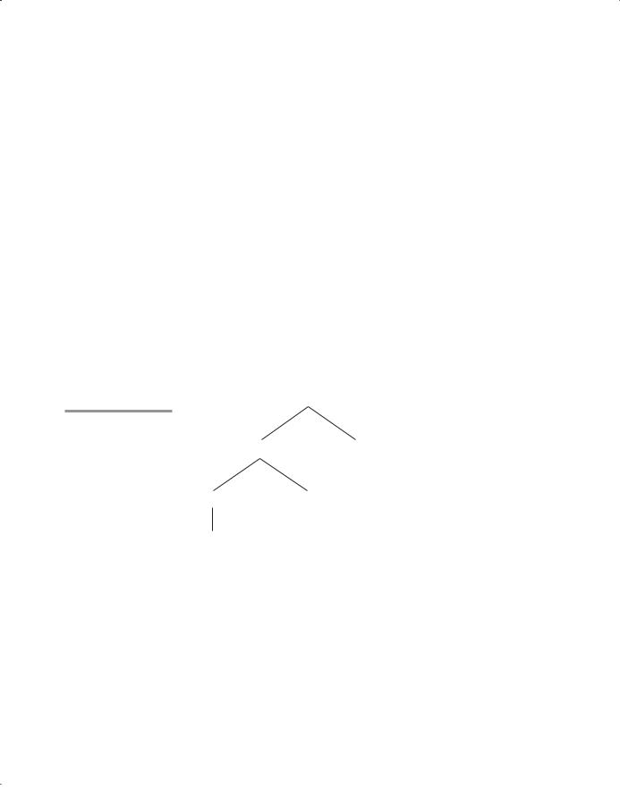
Figure 3.9
A parse tree of the binary number 110
3.5 Describing the Meanings of Programs: Dynamic Semantics |
143 |
construct. In denotational semantics, programming language constructs are mapped to mathematical objects, either sets or, more often, functions. However, unlike operational semantics, denotational semantics does not model the step-by-step computational processing of programs.
3.5.2.1 Two Simple Examples
We use a very simple language construct, character string representations of binary numbers, to introduce the denotational method. The syntax of such binary numbers can be described by the following grammar rules:
<bin_num> → '0'
|'1'
|<bin_num> '0' |<bin_num> '1'
A parse tree for the example binary number, 110, is shown in Figure 3.9. Notice that we put apostrophes around the syntactic digits to show they are not mathematical digits. This is similar to the relationship between ASCII coded digits and mathematical digits. When a program reads a number as a string, it must be converted to a mathematical number before it can be used as a value in the program.
<bin_num> |
|
<bin_num> |
'0' |
<bin_num> |
'1' |
'1'
The syntactic domain of the mapping function for binary numbers is the set of all character string representations of binary numbers. The semantic domain is the set of nonnegative decimal numbers, symbolized by N.
To describe the meaning of binary numbers using denotational semantics, we associate the actual meaning (a decimal number) with each rule that has a single terminal symbol as its RHS.
In our example, decimal numbers must be associated with the first two grammar rules. The other two grammar rules are, in a sense, computational rules, because they combine a terminal symbol, to which an object can be associated, with a nonterminal, which can be expected to represent some construct. Presuming an evaluation that progresses upward in the parse tree,
144 |
Chapter 3 Describing Syntax and Semantics |
the nonterminal in the right side would already have its meaning attached. So, a syntax rule with a nonterminal as its RHS would require a function that computed the meaning of the LHS, which represents the meaning of the complete RHS.
The semantic function, named Mbin, maps the syntactic objects, as described in the previous grammar rules, to the objects in N, the set of nonnegative decimal numbers. The function Mbin is defined as follows:
Mbin('0') = 0
Mbin('1') = 1
Mbin(<bin_num> '0') = 2 * Mbin(<bin_num>)
Mbin(<bin_num> '1') = 2 * Mbin(<bin_num>) + 1
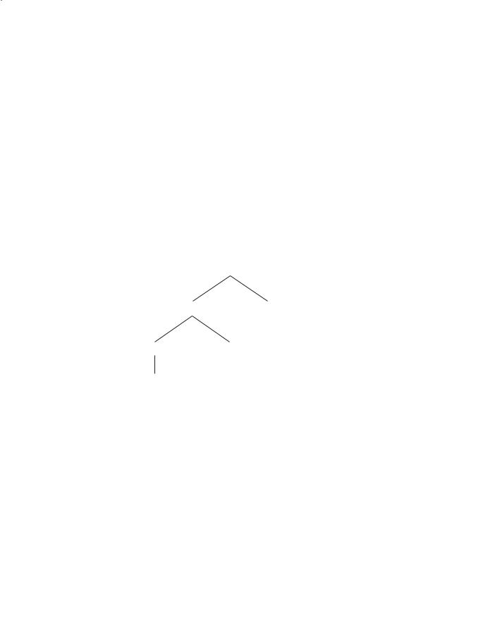
The meanings, or denoted objects (which in this case are decimal numbers), can be attached to the nodes of the parse tree shown on the previous page, yielding the tree in Figure 3.10. This is syntax-directed semantics. Syntactic entities are mapped to mathematical objects with concrete meaning.
Figure 3.10 |
6 |
|
|
|
|
<bin_num> |
|
A parse tree with |
|
|
|
denoted objects for 110 |
|
|
|
3 |
|
'0' |
|
|
<bin_num> |
||
|
1<bin_num> |
'1' |
|
'1' |
|
|
|
In part because we need it later, we now show a similar example for describing the meaning of syntactic decimal literals. In this case, the syntactic domain is the set of character string representations of decimal numbers. The semantic domain is once again the set N.
<dec_num> → '0'|'1'|'2'|'3'|'4'|'5'|'6'|'7''8'|'9' |<dec_num> ('0'|'1'|'2'|'3'|'4'|'5'|'6'|'7'|'8'|'9')
The denotational mappings for these syntax rules are
Mdec('0') = 0, Mdec('1') = 1, Mdec('2') = 2, . . ., Mdec('9') = 9
Mdec(<dec_num> '0') = 10 * Mdec(<dec_num>) Mdec(<dec_num> '1') = 10 * Mdec(<dec_num>) + 1
. . .
Mdec(<dec_num> '9') = 10 * Mdec(<dec_num>) + 9

3.5 Describing the Meanings of Programs: Dynamic Semantics |
145 |
In the following sections, we present the denotational semantics descriptions of a few simple constructs. The most important simplifying assumption made here is that both the syntax and static semantics of the constructs are correct. In addition, we assume that only two scalar types are included: integer and Boolean.
3.5.2.2 The State of a Program
The denotational semantics of a program could be defined in terms of state changes in an ideal computer. Operational semantics are defined in this way, and denotational semantics are defined in nearly the same way. In a further simplification, however, denotational semantics is defined in terms of only the values of all of the program’s variables. So, denotational semantics uses the state of the program to describe meaning, whereas operational semantics uses the state of a machine. The key difference between operational semantics and denotational semantics is that state changes in operational semantics are defined by coded algorithms, written in some programming language, whereas in denotational semantics, state changes are defined by mathematical functions.
Let the state s of a program be represented as a set of ordered pairs, as follows:
s = {<i1, v1>, <i2, v2>, . . . , <in, vn>}
Each i is the name of a variable, and the associated v’s are the current values of those variables. Any of the v’s can have the special value undef, which indicates that its associated variable is currently undefined. Let VARMAP be a function of two parameters: a variable name and the program state. The value of VARMAP (ij, s) is vj (the value paired with ij in state s). Most semantics mapping functions for programs and program constructs map states to states. These state changes are used to define the meanings of programs and program constructs. Some language constructs—for example, expressions—are mapped to values, not states.
3.5.2.3 Expressions
Expressions are fundamental to most programming languages. We assume here that expressions have no side effects. Furthermore, we deal with only very simple expressions: The only operators are + and *, and an expression can have at most one operator; the only operands are scalar integer variables and integer literals; there are no parentheses; and the value of an expression is an integer. Following is the BNF description of these expressions:
<expr> → <dec_num> | <var> | <binary_expr> <binary_expr> → <left_expr> <operator> <right_expr> <left_expr> → <dec_num> | <var>
<right_expr> → <dec_num> | <var> <operator> → + | *

146 |
Chapter 3 Describing Syntax and Semantics |
The only error we consider in expressions is a variable having an undefined value. Obviously, other errors can occur, but most of them are machinedependent. Let Z be the set of integers, and let error be the error value. Then Z h {error} is the semantic domain for the denotational specification for our expressions.
The mapping function for a given expression E and state s follows. To distinguish between mathematical function definitions and the assignment statements of programming languages, we use the symbol = to define mathematical functions. The implication symbol, =>, used in this definition connects the form of an operand with its associated case (or switch) construct. Dot notation is used to refer to the child nodes of a node. For example, <binary_expr>.<left_expr> refers to the left child node of <binary_expr>.
Me(<expr>, s) = case <expr> of
<dec_num>=>Mdec(<dec_num>, s) <var> =>if VARMAP(<var>, s) == undef
then error
else VARMAP(<var>, s) <binary_expr> =>
if(Me(<binary_expr>.<left_expr>,s) == undef OR Me(<binary_expr>.<right_expr>, s) == undef)
then error
else if (<binary_expr>.<operator> == '+')
then Me(<binary_expr>.<left_expr>, s) + Me(<binary_expr>.<right_expr>, s)
else Me(<binary_expr>.<left_expr>, s) * Me(<binary_expr>.<right_expr>, s)
3.5.2.4 Assignment Statements
An assignment statement is an expression evaluation plus the setting of the target variable to the expression’s value. In this case, the meaning function maps a state to a state. This function can be described with the following:
Ma(x = E, s) = if Me(E, s) == error then error
else s = {<i1, v1 >, <i2, v2 >, . . . , <in, vn >}, where for j = 1, 2, . . . , n
if ij == x
then vj = Me(E, s)
else vj = VARMAP(ij, s)
Note that the comparison in the third last line above, ij == x, is of names, not values.

3.5 Describing the Meanings of Programs: Dynamic Semantics |
147 |
3.5.2.5 Logical Pretest Loops
The denotational semantics of a logical pretest loop is deceptively simple. To expedite the discussion, we assume that there are two other existing mapping functions, Msl and Mb, that map statement lists and states to states and Boolean expressions to Boolean values (or error), respectively. The function is
Ml(while B do L, s) = if Mb(B, s) == undef then error
else if Mb(B, s) == false then s
else if Msl(L, s) == error then error
else Ml(while B do L, Msl(L, s))
The meaning of the loop is simply the value of the program variables after the statements in the loop have been executed the prescribed number of times, assuming there have been no errors. In essence, the loop has been converted from iteration to recursion, where the recursion control is mathematically defined by other recursive state mapping functions. Recursion is easier to describe with mathematical rigor than iteration.
One significant observation at this point is that this definition, like actual program loops, may compute nothing because of nontermination.
3.5.2.6 Evaluation
Objects and functions, such as those used in the earlier constructs, can be defined for the other syntactic entities of programming languages. When a complete system has been defined for a given language, it can be used to determine the meaning of complete programs in that language. This provides a framework for thinking about programming in a highly rigorous way.
As stated previously, denotational semantics can be used as an aid to language design. For example, statements for which the denotational semantic description is complex and difficult may indicate to the designer that such statements may also be difficult for language users to understand and that an alternative design may be in order.
Because of the complexity of denotational descriptions, they are of little use to language users. On the other hand, they provide an excellent way to describe a language concisely.
Although the use of denotational semantics is normally attributed to Scott and Strachey (1971), the general denotational approach to language description can be traced to the nineteenth century (Frege, 1892).

148 |
Chapter 3 Describing Syntax and Semantics |
3.5.3 Axiomatic Semantics
Axiomatic semantics, thus named because it is based on mathematical logic, is the most abstract approach to semantics specification discussed in this chapter. Rather than directly specifying the meaning of a program, axiomatic semantics specifies what can be proven about the program. Recall that one of the possible uses of semantic specifications is to prove the correctness of programs.
In axiomatic semantics, there is no model of the state of a machine or program or model of state changes that take place when the program is executed. The meaning of a program is based on relationships among program variables and constants, which are the same for every execution of the program.
Axiomatic semantics has two distinct applications: program verification and program semantics specification. This section focuses on program verification in its description of axiomatic semantics.
Axiomatic semantics was defined in conjunction with the development of an approach to proving the correctness of programs. Such correctness proofs, when they can be constructed, show that a program performs the computation described by its specification. In a proof, each statement of a program is both preceded and followed by a logical expression that specifies constraints on program variables. These, rather than the entire state of an abstract machine (as with operational semantics), are used to specify the meaning of the statement. The notation used to describe constraints—indeed, the language of axiomatic semantics—is predicate calculus. Although simple Boolean expressions are often adequate to express constraints, in some cases they are not.
When axiomatic semantics is used to specify formally the meaning of a statement, the meaning is defined by the statement’s effect on assertions about the data affected by the statement.
3.5.3.1 Assertions
The logical expressions used in axiomatic semantics are called predicates, or assertions. An assertion immediately preceding a program statement describes the constraints on the program variables at that point in the program. An assertion immediately following a statement describes the new constraints on those variables (and possibly others) after execution of the statement. These assertions are called the precondition and postcondition, respectively, of the statement. For two adjacent statements, the postcondition of the first serves as the precondition of the second. Developing an axiomatic description or proof of a given program requires that every statement in the program has both a precondition and a postcondition.
In the following sections, we examine assertions from the point of view that preconditions for statements are computed from given postconditions, although it is possible to consider these in the opposite sense. We assume all variables are integer type. As a simple example, consider the following assignment statement and postcondition:
sum = 2 * x + 1 {sum > 1}
3.5 Describing the Meanings of Programs: Dynamic Semantics |
149 |
Precondition and postcondition assertions are presented in braces to distinguish them from parts of program statements. One possible precondition for this statement is {x > 10}.
In axiomatic semantics, the meaning of a specific statement is defined by its precondition and its postcondition. In effect, the two assertions specify precisely the effect of executing the statement.
In the following subsections, we focus on correctness proofs of statements and programs, which is a common use of axiomatic semantics. The more general concept of axiomatic semantics is to state precisely the meaning of statements and programs in terms of logic expressions. Program verification is one application of axiomatic descriptions of languages.
3.5.3.2 Weakest Preconditions
The weakest precondition is the least restrictive precondition that will guarantee the validity of the associated postcondition. For example, in the statement and postcondition given in Section 3.5.3.1, {x > 10}, {x > 50}, and {x > 1000} are all valid preconditions. The weakest of all preconditions in this case is {x > 0}.
If the weakest precondition can be computed from the most general postcondition for each of the statement types of a language, then the processes used to compute these preconditions provide a concise description of the semantics of that language. Furthermore, correctness proofs can be constructed for programs in that language. A program proof is begun by using the characteristics of the results of the program’s execution as the postcondition of the last statement of the program. This postcondition, along with the last statement, is used to compute the weakest precondition for the last statement. This precondition is then used as the postcondition for the second last statement. This process continues until the beginning of the program is reached. At that point, the precondition of the first statement states the conditions under which the program will compute the desired results. If these conditions are implied by the input specification of the program, the program has been verified to be correct.
An inference rule is a method of inferring the truth of one assertion on the basis of the values of other assertions. The general form of an inference rule is as follows:
S1, S2, c, Sn
S
This rule states that if S1, S2, . . . , and Sn are true, then the truth of S can be inferred. The top part of an inference rule is called its antecedent; the bottom part is called its consequent.
An axiom is a logical statement that is assumed to be true. Therefore, an axiom is an inference rule without an antecedent.
For some program statements, the computation of a weakest precondition from the statement and a postcondition is simple and can be specified by an

150 |
Chapter 3 Describing Syntax and Semantics |
axiom. In most cases, however, the weakest precondition can be specified only by an inference rule.
To use axiomatic semantics with a given programming language, whether for correctness proofs or for formal semantics specifications, either an axiom or an inference rule must exist for each kind of statement in the language. In the following subsections, we present an axiom for assignment statements and inference rules for statement sequences, selection statements, and logical pretest loop statements. Note that we assume that neither arithmetic nor Boolean expressions have side effects.
3.5.3.3 Assignment Statements
The precondition and postcondition of an assignment statement together define precisely its meaning. To define the meaning of an assignment statement, given a postcondition, there must be a way to compute its precondition from that postcondition.
Let x = E be a general assignment statement and Q be its postcondition. Then, its precondition, P, is defined by the axiom
P = QxSE
which means that P is computed as Q with all instances of x replaced by E. For example, if we have the assignment statement and postcondition
a = b / 2 - 1 {a < 10}
the weakest precondition is computed by substituting b / 2 - 1 for a in the postcondition {a < 10}, as follows:
b / 2 - 1 < 10 b < 22
Thus, the weakest precondition for the given assignment statement and postcondition is {b < 22}. Remember that the assignment axiom is guaranteed to be correct only in the absence of side effects. An assignment statement has a side effect if it changes some variable other than its target.
The usual notation for specifying the axiomatic semantics of a given statement form is
{P}S{Q}
where P is the precondition, Q is the postcondition, and S is the statement form. In the case of the assignment statement, the notation is
{QxSE} x = E{Q}

3.5 Describing the Meanings of Programs: Dynamic Semantics |
151 |
As another example of computing a precondition for an assignment statement, consider the following:
x = 2 * y - 3 {x > 25}
The precondition is computed as follows:
2 * y - 3 > 25 y > 14
So {y > 14} is the weakest precondition for this assignment statement and postcondition.
Note that the appearance of the left side of the assignment statement in its right side does not affect the process of computing the weakest precondition. For example, for
x = x + y - 3 {x > 10}
the weakest precondition is
x + y - 3 > 10
y > 13 - x
Recall that axiomatic semantics was developed to prove the correctness of programs. In light of that, it is natural at this point to wonder how the axiom for assignment statements can be used to prove anything. Here is how: A given assignment statement with both a precondition and a postcondition can be considered a logical statement, or theorem. If the assignment axiom, when applied to the postcondition and the assignment statement, produces the given precondition, the theorem is proved. For example, consider the logical statement
{x > 3} x = x - 3 {x > 0}
Using the assignment axiom on
x = x - 3 {x > 0}
produces {x > 3}, which is the given precondition. Therefore, we have proven the example logical statement.
Next, consider the logical statement
{x > 5} x = x - 3 {x > 0}
In this case, the given precondition, {x > 5}, is not the same as the assertion produced by the axiom. However, it is obvious that {x > 5} implies {x > 3}.

152 Chapter 3 Describing Syntax and Semantics
To use this in a proof, an inference rule, named the rule of consequence, is needed. The form of the rule of consequence is
{P} S {Q}, P => P, Q =>Q
{P } S {Q }
The => symbol means “implies,” and S can be any program statement. The rule can be stated as follows: If the logical statement {P} S {Q} is true, the assertion P implies the assertion P, and the assertion Q implies the assertion Q , then it can be inferred that {P } S {Q }. In other words, the rule of consequence says that a postcondition can always be weakened and a precondition can always be strengthened. This is quite useful in program proofs. For example, it allows the completion of the proof of the last logical statement example above. If we let P be {x > 3}, Q and Q be {x > 0}, and P be {x > 5}, we have
{x>3}x = x–3{x>0},(x>5) => {x>3},(x>0) => (x>0)
{x>5}x = x–3{x>0}
The first term of the antecedent ({x > 3} x = x – 3 {x > 0}) was proven with the assignment axiom. The second and third terms are obvious. Therefore, by the rule of consequence, the consequent is true.
3.5.3.4 Sequences
The weakest precondition for a sequence of statements cannot be described by an axiom, because the precondition depends on the particular kinds of statements in the sequence. In this case, the precondition can only be described with an inference rule. Let S1 and S2 be adjacent program statements. If S1 and S2 have the following preand postconditions
{P1} S1 {P2} {P2} S2 {P3}
the inference rule for such a two-statement sequence is
{P1} S1 {P2}, {P2} S2 {P3}
{P1} S1, S2 {P3}
So, for our example, {P1} S1; S2 {P3} describes the axiomatic semantics of the sequence S1; S2. The inference rule states that to get the sequence precondition, the precondition of the second statement is computed. This new assertion is then used as the postcondition of the first statement, which can then be used to compute the precondition of the first statement, which is also the precondition of the whole sequence. If S1 and S2 are the assignment statements

3.5 Describing the Meanings of Programs: Dynamic Semantics |
153 |
x1= E1
and
x2= E2
then we have
{P3x2SE2} x2= E2 {P3}
{(P3x2SE2)x1SE1} x1= E1 {P3x2SE2}
Therefore, the weakest precondition for the sequence x1 = E1; x2 = E2 with postcondition P3 is {(P3x2SE2)x1SE1}.
For example, consider the following sequence and postcondition:
y = 3 * x + 1;
x = y + 3;
{x < 10}
The precondition for the second assignment statement is
y < 7
which is used as the postcondition for the first statement. The precondition for the first assignment statement can now be computed:
3 * x + 1 < 7 x < 2
So, {x < 2} is the precondition of both the first statement and the twostatement sequence.
3.5.3.5 Selection
We next consider the inference rule for selection statements, the general form of which is
if B then S1 else S2
We consider only selections that include else clauses. The inference rule is
{B and P} S1 {Q}, {(not B) and P} S2{Q}
{P} if B then S1 else S2 {Q}
This rule indicates that selection statements must be proven both when the Boolean control expression is true and when it is false. The first logical statement above the line represents the then clause; the second represents the else

154 |
Chapter 3 Describing Syntax and Semantics |
clause. According to the inference rule, we need a precondition P that can be used in the precondition of both the then and else clauses.
Consider the following example of the computation of the precondition using the selection inference rule. The example selection statement is
if x > 0 then
y = y - 1
else
y = y + 1
Suppose the postcondition, Q, for this selection statement is {y > 0}. We can use the axiom for assignment on the then clause
y = y - 1 {y > 0}
This produces {y - 1 > 0} or {y > 1}. It can be used as the P part of the precondition for the then clause. Now we apply the same axiom to the else clause
y = y + 1 {y > 0}
which produces the precondition {y + 1 > 0} or {y > -1}. Because {y > 1} => {y > -1}, the rule of consequence allows us to use {y > 1} for the precondition of the whole selection statement.
3.5.3.6 Logical Pretest Loops
Another essential construct of imperative programming languages is the logical pretest, or while loop. Computing the weakest precondition for a while loop is inherently more difficult than for a sequence, because the number of iterations cannot always be predetermined. In a case where the number of iterations is known,
the loop can be unrolled and treated as a sequence.
The problem of computing the weakest precondition for loops is similar to the problem of proving a theorem about all positive integers. In the latter case, induction is normally used, and the same inductive method can be used for some loops. The principal step in induction is finding an inductive hypothesis. The corresponding step in the axiomatic semantics of a while loop is finding an assertion called a loop invariant, which is crucial to finding the weakest precondition.
The inference rule for computing the precondition for a while loop is
{I and B} S {I}
{I} while B do S end {I and (not B)}
where I is the loop invariant. This seems simple, but it is not. The complexity lies in finding an appropriate loop invariant.

3.5 Describing the Meanings of Programs: Dynamic Semantics |
155 |
The axiomatic description of a while loop is written as
{P} while B do S end {Q}
The loop invariant must satisfy a number of requirements to be useful. First, the weakest precondition for the while loop must guarantee the truth of the loop invariant. In turn, the loop invariant must guarantee the truth of the postcondition upon loop termination. These constraints move us from the inference rule to the axiomatic description. During execution of the loop, the truth of the loop invariant must be unaffected by the evaluation of the loopcontrolling Boolean expression and the loop body statements. Hence, the name invariant.
Another complicating factor for while loops is the question of loop termination. A loop that does not terminate cannot be correct, and in fact computes nothing. If Q is the postcondition that holds immediately after loop exit, then a precondition P for the loop is one that guarantees Q at loop exit and also guarantees that the loop terminates.
The complete axiomatic description of a while construct requires all of the following to be true, in which I is the loop invariant:
P => I
{I and B} S {I}
(I and (not B)) => Q the loop terminates
If a loop computes a sequence of numeric values, it may be possible to find a loop invariant using an approach that is used for determining the inductive hypothesis when mathematical induction is used to prove a statement about a mathematical sequence. The relationship between the number of iterations and the precondition for the loop body is computed for a few cases, with the hope that a pattern emerges that will apply to the general case. It is helpful to treat the process of producing a weakest precondition as a function, wp. In general
wp(statement, postcondition) = precondition
A wp function is often called a predicate transformer, because it takes a predicate, or assertion, as a parameter and returns another predicate.
To find I, the loop postcondition Q is used to compute preconditions for several different numbers of iterations of the loop body, starting with none. If the loop body contains a single assignment statement, the axiom for assignment statements can be used to compute these cases. Consider the example loop:
while y <> x do y = y + 1 end {y = x}
Remember that the equal sign is being used for two different purposes here. In assertions, it means mathematical equality; outside assertions, it means the assignment operator.

156 |
Chapter 3 Describing Syntax and Semantics |
For zero iterations, the weakest precondition is, obviously,
{y = x}
For one iteration, it is
wp(y = y + 1, {y = x}) = {y + 1 = x}, or {y = x - 1}
For two iterations, it is
wp(y = y + 1, {y = x - 1})={y + 1 = x - 1}, or {y = x - 2}
For three iterations, it is
wp(y = y + 1, {y = x - 2})={y + 1 = x - 2}, or {y = x – 3}
It is now obvious that {y < x} will suffice for cases of one or more iterations. Combining this with {y = x} for the zero iterations case, we get {y <= x}, which can be used for the loop invariant. A precondition for the while statement can be determined from the loop invariant. In fact, I can be used as the precondition, P.
We must ensure that our choice satisfies the four criteria for I for our example loop. First, because P = I, P => I. The second requirement is that it must be true that
{I and B} S {I}
In our example, we have
{y <= x and y <> x} y = y + 1 {y <= x}
Applying the assignment axiom to
y = y + 1 {y <= x}
we get {y + 1 <= x}, which is equivalent to {y < x}, which is implied by {y <= x and y <> x}. So, the earlier statement is proven.
Next, we must have {I and (not B)} => Q
In our example, we have
{(y <= x) and not (y <> x)} => {y = x} {(y <= x) and (y = x)} => {y = x}
{y = x} => {y = x}
So, this is obviously true. Next, loop termination must be considered. In this example, the question is whether the loop
{y <= x} while y <> x do y = y + 1 end {y = x}

3.5 Describing the Meanings of Programs: Dynamic Semantics |
157 |
terminates. Recalling that x and y are assumed to be integer variables, it is easy to see that this loop does terminate. The precondition guarantees that y initially is not larger than x. The loop body increments y with each iteration, until y is equal to x. No matter how much smaller y is than x initially, it will eventually become equal to x. So the loop will terminate. Because our choice of I satisfies all four criteria, it is a satisfactory loop invariant and loop precondition.
The previous process used to compute the invariant for a loop does not always produce an assertion that is the weakest precondition (although it does in the example).
As another example of finding a loop invariant using the approach used in mathematical induction, consider the following loop statement:
while s > 1 do s = s / 2 end {s = 1}
As before, we use the assignment axiom to try to find a loop invariant and a precondition for the loop. For zero iterations, the weakest precondition is {s = 1}. For one iteration, it is
wp(s = s / 2, {s = 1}) = {s / 2 = 1}, or {s = 2}
For two iterations, it is
wp(s = s / 2, {s = 2}) = {s / 2 = 2}, or {s = 4}
For three iterations, it is
wp(s = s / 2, {s = 4}) = {s / 2 = 4}, or {s = 8}
From these cases, we can see clearly that the invariant is
{s is a nonnegative power of 2}
Once again, the computed I can serve as P, and I passes the four requirements. Unlike our earlier example of finding a loop precondition, this one clearly is not a weakest precondition. Consider using the precondition {s > 1}. The logical statement
{s > 1} while s > 1 do s = s / 2 end {s = 1}
can easily be proven, and this precondition is significantly broader than the one computed earlier. The loop and precondition are satisfied for any positive value for s, not just powers of 2, as the process indicates. Because of the rule of consequence, using a precondition that is stronger than the weakest precondition does not invalidate a proof.
Finding loop invariants is not always easy. It is helpful to understand the nature of these invariants. First, a loop invariant is a weakened version of the loop postcondition and also a precondition for the loop. So, I must be weak enough to be satisfied prior to the beginning of loop execution, but when combined with the loop exit condition, it must be strong enough to force the truth of the postcondition.

158 |
Chapter 3 Describing Syntax and Semantics |
Because of the difficulty of proving loop termination, that requirement is often ignored. If loop termination can be shown, the axiomatic description of the loop is called total correctness. If the other conditions can be met but termination is not guaranteed, it is called partial correctness.
In more complex loops, finding a suitable loop invariant, even for partial correctness, requires a good deal of ingenuity. Because computing the precondition for a while loop depends on finding a loop invariant, proving the correctness of programs with while loops using axiomatic semantics can be difficult.
3.5.3.7 Program Proofs
This section provides validations for two simple programs. The first example of a correctness proof is for a very short program, consisting of a sequence of three assignment statements that interchange the values of two variables.
{x = A AND y = B}
t = x;
x = y;
y = t;
{x = B AND y = A}
Because the program consists entirely of assignment statements in a sequence, the assignment axiom and the inference rule for sequences can be used to prove its correctness. The first step is to use the assignment axiom on the last statement and the postcondition for the whole program. This yields the precondition
{x = B AND t = A}
Next, we use this new precondition as a postcondition on the middle statement and compute its precondition, which is
{y = B AND t = A}
Next, we use this new assertion as the postcondition on the first statement and apply the assignment axiom, which yields
{y = B AND x = A}
which is the same as the precondition on the program, except for the order of operands on the AND operator. Because AND is a symmetric operator, our proof is complete.
The following example is a proof of correctness of a pseudocode program that computes the factorial function.
3.5 Describing the Meanings of Programs: Dynamic Semantics |
159 |
{n >= 0} count = n; fact = 1;
while count <> 0 do fact = fact * count; count = count - 1;
end
{fact = n!}
The method described earlier for finding the loop invariant does not work for the loop in this example. Some ingenuity is required here, which can be aided by a brief study of the code. The loop computes the factorial function in order of the last multiplication first; that is, (n - 1) * n is done first, assuming n is greater than 1. So, part of the invariant can be
fact = (count + 1) * (count + 2) *...* (n - 1) * n
But we must also ensure that count is always nonnegative, which we can do by adding that to the assertion above, to get
I = (fact = (count + 1) *...* n) AND (count >= 0)
Next, we must confirm that this I meets the requirements for invariants. Once again we let I also be used for P, so P clearly implies I. The next question is
{I and B} S {I}
I and B is
((fact = (count + 1) *...* n) AND (count >= 0)) AND
(count <> 0)
which reduces to
(fact = (count + 1) *...* n) AND (count > 0)
In our case, we must compute the precondition of the body of the loop, using the invariant for the postcondition. For
{P} count = count - 1 {I}
we compute P to be
{(fact = count * (count + 1) *...* n) AND (count >= 1)}

160 |
Chapter 3 Describing Syntax and Semantics |
Using this as the postcondition for the first assignment in the loop body,
{P} fact = fact * count {(fact = count * (count + 1) *...* n) AND (count >= 1)}
In this case, P is
{(fact = (count + 1) *...* n) AND (count >= 1)}
It is clear that I and B implies this P, so by the rule of consequence, {I AND B} S {I}
is true. Finally, the last test of I is I AND (NOT B) => Q
For our example, this is
((fact = (count + 1) *...* n) AND (count >= 0)) AND (count = 0)) => fact = n!
This is clearly true, for when count = 0, the first part is precisely the definition of factorial. So, our choice of I meets the requirements for a loop invariant. Now we can use our P (which is the same as I) from the while as the postcondition on the second assignment of the program
{P} fact = 1 {(fact = (count + 1) *...* n) AND (count >= 0)}
which yields for P
(1 = (count + 1) *...* n) AND (count >= 0))
Using this as the postcondition for the first assignment in the code
{P} count = n {(1 = (count + 1) *...* n) AND (count >= 0))}
produces for P
{(n + 1) *...* n = 1) AND (n >= 0)}
The left operand of the AND operator is true (because 1 = 1) and the right operand is exactly the precondition of the whole code segment, {n >= 0}. Therefore, the program has been proven to be correct.
3.5.3.8 Evaluation
As stated previously, to define the semantics of a complete programming language using the axiomatic method, there must be an axiom or an inference rule for each statement type in the language. Defining axioms or inference rules for