

Ceramic materials Carter Horton / fulltext 33 Using magnetic fields and storing data
.pdf33
Using Magnetic Fields and Storing Data
CHAPTER PREVIEW
If you were asked to give an example of a magnetic material instinctively you would probably say iron. It is a good example, but in its pure form iron is not a very useful magnet. Ceramics can be magnetic too and they were the first magnets known to humans. About 600,000 t of ceramic magnets are produced each year making them, in terms of volume, commercially more important than metallic magnets. The largest market segment is hard ferrites (permanent magnets) that are used in a range of applications including motors for electric toothbrushes and windshield wipers in automobiles, refrigerator door seals, speakers, and stripes on the back of the ubiquitous credit and ATM cards. Soft ferrites can be magnetized and demagnetized easily and are used in cell telephones, transformer cores, and, now to a somewhat lesser extent, magnetic recording.
Ferrite is a term used for ceramics that contain Fe2O3 as a principal component. Magnetism has probably fascinated more people, including Socrates and Mozart (listen to
Così fan tutte), over the years than any other materials property. For over four thousand years the strange power of magnets has captured our imagination. Yet it remains the least well understood of all properties. In this chapter we will start by describing some of the basic characteristics of magnetic materials, which often contain one of the first row transition metals, Fe, Co, or Ni. The electron arrangement in the 3d level of these atoms is the key. The manganates are a very interesting class of magnetic ceramic. Although they are not new, the recent discovery that they exhibit colossal magnetoresistance (just like the giant magnetoresistance observed in metal multilayers only much bigger) has renewed interest in these materials. Structurally the manganates are very similar to the high-temperature superconductors (HTSCs). The similarity may be more than coincidental.
33.1 A BRIEF HISTORY OF MAGNETIC CERAMICS
Applications of magnetism began with ceramics. The first magnetic material to be discovered was lodestone, which is better known now as magnetite (Fe3O4). In its naturally occurring state it is permanently magnetized and is the most magnetic mineral. The strange power of lodestone was well known in ancient times. In c. 400 BCE Socrates dangled iron rings beneath a piece of lodestone and found that the lodestone enabled the rings to attract other rings. They had become magnetized. Even earlier ( c. 2600 BCE) a Chinese legend tells of the Emperor Hwang-ti being guided into battle through a dense fog by means of a small pivoting figure with a piece of lodestone embedded in its outstretched arm. The figure always pointed south and was probably the first compass. The term lodestone was coined by the British from the old English word lode, which meant to lead or guide.
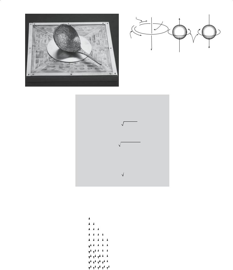
Figure 33.1 shows an ancient Chinese compass. The spoon or ladle was carved out of lodestone and rests on a
polished bronze plate. The rounded bottom of the spoon swivels on the plate until it points south. Although this compass has been found to work it was used apparently for quasimagical rather than navigational purposes.
Magnetite is found in many parts of the world and is an important iron ore used for steel making. The word magnet comes from the Greek word magnes, which itself may derive from the ancient colony of Magnesia (in Turkey). Magnetite was mined in Magnesia 2500 years ago. Today, large deposits of magnetite are found at Kiruna in Sweden and in the Adirondack region of New York.
Commercial interest in ceramic magnets really started in the early 1930s with the filing of a Japanese patent describing applications of copper and cobalt ferrites. In 1947 J.L. Snoeck of N.V. Philips Gloeilampenfabrieken performed a detailed study of ferrites, and the following year Louis Néel published his theory of ferrimagnetism. This latter study was particularly important because most of the ceramics that have useful magnetic properties are ferrimagnetic. The first commercial ceramic magnets were produced in 1952 by researchers at the Philips Company,
598 .............................................................................................................. |
U S I N G M A G N E T I C F I E L D S A N D S T O R I N G D A T A |
Direction of |
N |
|
|
current |
Nucleus |
|
|
e- |
|
|
|
+ |
e- |
or |
e- |
Direction of |
|
|
|
electron motion |
|
Direction of |
|
|
|
electron spin |
|
N |
|
|
N |
|
|
|
|
(A) |
(B) |
|
|
FIGURE 33.2 Generation of atomic magnetic moments by
(a) electron orbital motion around the nucleus; (b) electron spin around its axis of rotation.
netic dipoles are small internal magnets with north and south poles.
FIGURE 33.1 An ancient Chinese compass.
the same company that introduced the compact audiocassette in 1963.
33.2 MAGNETIC DIPOLES
The Danish physicist Hans Christian Oersted discovered that an electric current (i.e., moving electrons) gives rise to a magnetic force. In an atom, there are two possible sources of electron motion that can create a magnetic dipole and produce the resultant macroscopic magnetic properties of a material. Mag-
MAGNETIC MOMENTS
The fundamental magnetic moment is the Bohr magneton, μB, which has a value of 9.27 × 10⁻²⁴ A·m2.
The orbital magnetic moment, μorb, of a single electron is
μorb = μB [l (l + 1)] |
(Box 33.1) |
l is the orbital shape quantum number (see Chapter 3). The spin magnetic moment of an electron is
μs = 2μB [ms (ms + 1)] |
(Box 33.2) |
In ceramics where the magnetic behavior is due to the presence of transition metal ions with unpaired electron spins in the 3d orbital the magnetic moment of the ion due to electron spin, μion, is
μion = 2μB [S (S + 1)] |
(Box 33.3) |
S = ∑ ms
Orbital motion. Equivalent to a small current loop generating a very small magnetic field. The direction of the magnetic moment is along the orbit axis as illustrated in Figure 33.2a.
Spin. Origin of the fourth quantum number,
ms, that we used in Chapter 3. The magnetic moment is along the spin axis as shown in
Figure 33.2b and will be either up (ms = +1/2) or
in an antiparallel down direction (ms = −1/2).
The magnetic moment due to electron spin is, when present, dominant
TABLE 33.1 Magnetic Moments of Isolated Transition Metal Cations |
|
||||||||||||||||||
|
|
|
|
|
|
|
|
|
|
|
|
|
|
|
|
|
|
Calculated moments |
Measured |
Cations |
Electronic configuration |
using Eq. B3 |
moments (mB) |
||||||||||||||||
|
|
|
|
|
|
|
|
|
|
|
|
|
|
|
|
|
|
|
|
Sc3+, Ti4+ |
3d0 |
|
|
|
|
|
|
|
|
|
|
|
|
|
|
|
|
0.00 |
0.0 |
|
|
|
|
|
|
|
|
|
|
|
|
|
|
|
|
||||
|
|
|
|
|
|
|
|
|
|
|
|
|
|
|
|
||||
V4+, Ti3+ |
3d1 |
|
|
|
|
|
|
|
|
|
|
|
|
|
|
|
|
1.73 |
1.8 |
|
|
|
|
|
|
|
|
|
|
|
|
|
|
|
|
||||
V3+ |
|
|
|
|
|
|
|
|
|
|
|
|
|||||||
3d2 |
|
|
|
|
|
|
|
|
|
|
|
|
|
|
|
|
2.83 |
2.8 |
|
|
|
|
|
|
|
|
|
|
|
|
|
|
|
|
|
||||
V2+, Cr3+ |
|
|
|
|
|
|
|
|
|
|
|
||||||||
3d3 |
|
|
|
|
|
|
|
|
|
|
|
|
|
|
|
3.87 |
3.8 |
||
|
|
|
|
|
|
|
|
|
|
|
|
|
|
|
|
||||
Mn3+, Cr2+ |
|
|
|
|
|
|
|
|
|
|
|||||||||
3d4 |
|
|
|
|
|
|
|
|
|
|
|
|
|
|
4.90 |
4.9 |
|||
|
|
|
|
|
|
|
|
|
|
|
|
|
|
|
|
||||
Mn2+, Fe3+ |
|
|
|
|
|
|
|
|
|
||||||||||
3d5 |
|
|
|
|
|
|
|
|
|
|
|
|
|
5.92 |
5.9 |
||||
|
|
|
|
|
|
|
|
|
|
|
|
|
|
|
|
||||
Fe2+ |
|
|
|
|
|
|
|
|
|||||||||||
3d6 |
|
|
|
|
|
|
|
|
|
|
|
|
4.90 |
5.4 |
|||||
|
|
|
|
|
|
|
|
|
|
|
|
|
|
|
|
||||
Co2+ |
|
|
|
|
|
|
|
||||||||||||
3d7 |
|
|
|
|
|
|
|
|
|
|
|
|
|
3.87 |
4.8 |
||||
|
|
|
|
|
|
|
|
|
|
|
|
|
|
|
|
||||
Ni2+ |
|
|
|
|
|
|
|||||||||||||
3d8 |
|
|
|
|
|
|
|
|
|
|
|
|
|
2.83 |
3.2 |
||||
|
|
|
|
|
|
|
|
|
|
|
|
|
|
|
|
||||
Cu2+ |
|
|
|
|
|
||||||||||||||
3d9 |
|
|
|
|
|
|
|
|
|
|
|
|
|
1.73 |
1.9 |
||||
|
|
|
|
|
|
|
|
|
|
|
|
|
|
|
|
||||
Cu+, Zn2+ |
|
|
|
|
|||||||||||||||
3d10 |
|
|
|
|
|
|
|
|
|
|
|
|
|
0.00 |
0.0 |
||||
|
|
|
|
|
|
|
|
|
|
|
|
|
|
|
|
||||
|
|
|
|
|
|
|
|
|
|
|
|
|
|
|
|
|
|
|
|
3 3 . 2 M A G N E T I C D I P O L E S ................................................................................................................................................ |
599 |
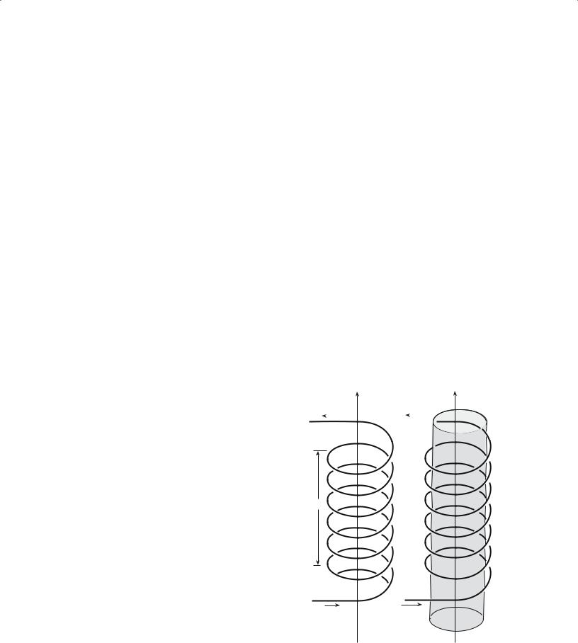
TABLE 33.2 Terms and Units Used in Magnetism |
|
|
|
Parameter |
Definition |
Units/value |
Conversion factor |
|
|
|
|
H |
Magnetic field strength |
A/m |
1 A/m = 4π × 10−3 oersted (Oe) |
Hc |
Coercive field |
A/m |
|
Hcr |
Critical field |
A/m |
|
M |
Magnetization |
A/m |
|
B |
Magnetic flux density |
T |
T = Wb m−2 = kg A−1 s2 = V s m−2 |
|
Magnetic induction |
|
= 104 gauss (G) |
μo |
Permeability of a vacuum |
4π × 10−7 H/m |
1 H = 1 J s2 C−2 |
μ |
Permeability |
H/m |
1 H/m = 1 Wb m−1 A−1 |
μr |
Relative permeability |
Dimensionless |
|
χ |
Susceptibility |
Dimensionless |
|
μion |
Net magnetic moment of an atom or ion |
A·m2 |
|
μs |
Spin magnetic moment |
A·m2 |
|
μorb |
Orbital magnetic moment |
A·m2 |
|
μB |
Bohr magneton |
9.274 × 10⁻²⁴ A·m2 |
|
θc |
Curie temperature |
K |
0 K = −273°C |
θN |
Néel temperature |
K |
|
Tc |
Critical temperature for superconductivity |
K |
|
C |
Curie constant |
K |
|
|
|
|
|
over that due to orbital motion. Table 33.1 lists values of μion calculated for some first row transition metal ions using Eq. Box 33.3. You can see that, in general, the calculated values agree well with the experimental values. This agreement shows that we are justified in considering only the contribution of the spin magnetic moment to the overall magnetic moment.
When an electron orbital in an atom is filled, i.e., all the electrons are paired up, both the orbital magnetic moment and the spin magnetic moment are zero.
33.3 THE BASIC EQUATIONS, THE WORDS, AND THE UNITS
Table 33.2 lists the important parameters used in this chapter and their units. The situation regarding units is more complicated for magnetism than for almost any other property. The reason is that some of the older units, in particular the oersted (Oe) and the gauss (G), are still in widespread use despite being superceded, in the SI system, by A/m and T, respectively.
The properties of most interest to us in the description of magnetic behavior are
μ
χ
These terms are, of course, related to each other and by considering the role of H to macroscopic measures such as M and B.
The usual starting point to arrive at expressions for μ and χ is to consider a coil of wire in a vacuum as illustrated in Figure 33.3a. A current, I, passed through the wire generates a magnetic field H
H = IN |
(33.1) |
where N is the number of turns of wire per meter. The magnetic induction or magnetic flux density, B, is related to H by
B = μ0H |
(33.2) |
μo is a universal constant.
When a material is placed inside the coil, as shown in Figure 33.3b, it becomes “magnetized.” The magnetic
I |
|
|
I |
|
|
|
|
|
|
l
N turns |
|
I |
I |
(A) |
(B) |
FIGURE 33.3 Generation of a magnetic field by current flowing in a coil of wire (a) in a vacuum; (b) with a material present.
600 .............................................................................................................. |
U S I N G M A G N E T I C F I E L D S A N D S T O R I N G D A T A |

moment produced in the material by the external field changes B:
B = μ0H + μ0M |
(33.3) |
M represents the response of the material to H, which is linear, and the ratio gives
χ = M/H |
(33.4) |
By simple substitution we get |
|
B = μ0(1 + χ)H |
(33.5) |
B/H is then the permeability: |
|
B/H = μ0(1 + χ) = μ |
(33.6) |
The ratio of the permeabilities gives us the relative permeability:
μ |
= 1 + χ = μr |
(33.7) |
μ0
There are many qualitative similarities between magnetic parameters and those we used to describe dielectrics in Chapter 31. In the former case, the material is responding to an applied magnetic field, and in the latter case, it is
responding to an applied electric field.
H and the electric field strength ξ (V/m). Both are the external driving force, which causes the orientation of either magnetic or electric dipoles resulting in magnetization or polarization, respectively.
B and the polarization P (C/m2). Both correspond to the total field after dipole orientation.
χ and dielectric constant, κ. Both are dimensionless “constants” that describe the magnitude of a material’s response to the applied field. They are both properties of a material and depend on the types of atoms, the interatomic bonding, and, the crystal structure.
μo and the permittivity of a vacuum ε0 are constants.
They are reference values to establish the strength of a materials response to H or ξ, respectively.
The similarities described above are not surprising. In both cases, we are con-
cerned with the relationship between an external field and the dipoles within a material. Despite these similarities the physical
nature of the dipoles and their origin is very different. In the case of a dielectric, the dipoles are electric; there is a separation of positive and negative charges. These dipoles can be permanent or induced. In a magnetic material, the dipoles are, of course, magnetic in origin and are due to electron motion.
A note on terminology: In most materials science textbooks, as we have done here, H is defined as the magnetic field or the applied magnetic field and B as the magnetic flux density. In many physics textbooks B is referred to as the magnetic field and H is often ignored. The physics convention is adopted for purely historical reasons, but it does have the advantage of reducing the number of terms we need to consider. Also H has nothing to do with a material whereas B is a measure of the response of a material to an applied magnetic field. Another point to note is that B and H are both vector quantities and because the magnetic properties of a material are anisotropic (different along different directions in the crystal) they should actually be represented by a second-rank tensor.
33.4 THE FIVE CLASSES OF MAGNETIC MATERIAL
There are five main types of magnetic behavior and these can be divided into two general categories:
Induced
Spontaneous
Table 33.3 summarizes the properties of the five classes. We can find examples of each in ceramics.
33.5 DIAMAGNETIC CERAMICS
Most ceramics are diamagnetic. The reason is that all the electrons are paired during bond formation and as a result the net magnetic moment due to electron spin is zero. Table 33.4 lists χ for several diamagnetic materials. Cu, Au, and Ag are diamagnetic even though their atoms have unpaired valence electrons. When the atoms combine to form the metal the valence electrons are shared by the crystal as a whole (to form the electron gas) and, on average, there will be as many electrons with ms = +1/2 as with ms = −1/2.
Most diamagnetic ceramics are of no commercial significance and of little scientific interest, at least not for their magnetic behavior.
The one exception is the ceramic superconductors, which are perfect diamagnets below a critical magnetic field.
3 3 . 5 D I A M A G N E T I C C E R A M I C S ........................................................................................................................................ |
601 |

TABLE 33.3 Magnetic Classification of Materials |
|
|
|
|
|
Critical |
Temperature |
Spontaneous |
|
Class |
temperature c |
variation of c |
magnetization |
Structure on atomic scale |
Diamagnetic |
None |
−10−6 |
to −10−5 |
Paramagnetic |
None |
+10−5 |
to +10−3 |
Ferromagnetic |
θC |
Large (below θC) |
|
Antiferromagnetic |
θN |
As paramagnetic |
|
Ferrimagnetic |
θC |
As ferromagnetic |
Constant |
None |
Atoms have no permanent dipole |
|
|
moments |
χ = C /T |
None |
Atoms have permanent dipole |
|
|
moments; neighboring moments |
|
|
do not interact |
Above θC, |
Below θC, Ms(T )/Ms(0) |
Atoms have permanent dipole |
χ = C /(T − θ), |
against T/θC follows a |
moments; interaction produces |
with θ ≈ θC |
universal curve; above |
parallel alignment |
Above θN, |
θC, none |
|
None |
Atoms have permanent dipole |
|
χ = C /(T ± θ), |
|
moments; interaction produces |
with θ ≠ θN, |
|
antiparallel alignment |
below θN, χ |
|
|
decreases, |
|
|
anisotropic |
|
|
Above θC, |
Below θC, does not |
Atoms have permanent dipole |
χ ≈ C /(T ± θ), |
follow universal curve; |
moments; interaction produces |
with θ ≠ θC |
above θC, none |
antiparallel alignment; moments |
|
|
are not equal |
33.6 SUPERCONDUCTING MAGNETS
When a superconductor in its normal (i.e., nonsuperconducting) state is placed in a magnetic field and then cooled below its critical temperature the induced
magnetization, |
M, |
exactly |
opposes H and so from Eq. |
||
33.3, we can write |
|
|
B = 0 |
|
(33.8) |
TABLE 33.4 Magnetic Susceptibilities for Several
Diamagnetic Materials
Material |
c (ppm) |
|
|
Al2O3 |
−37.0 |
Be |
−9.0 |
BeO |
−11.9 |
Bi |
−280.1 |
B |
−6.7 |
CaO |
−15.0 |
CaF2 |
−28.0 |
C (diamond) |
−5.9 |
C (graphite) |
−6.0 |
Cu |
−5.5 |
Ge |
−76.8 |
Au |
−28.0 |
Pb |
−23.0 |
LiF |
−10.1 |
MgO |
−10.2 |
Si |
−3.9 |
Ag |
−19.5 |
NaCl |
−30.3 |
|
|
The net effect is that the whole of the magnetic flux appears to have been suddenly ejected from the material and it behaves as a perfect diamagnet. This phenomenon is known as the Meissner effect and is usually demonstrated by suspending a magnet above a cooled pellet of the superconductor.
There is an upper limit to the strength of the magnetic field that can be applied to a superconductor without changing its
diamagnetic behavior. At a critical field Hcr the magnetization goes toward zero and the material reverts to its normal state. For most elemental superconductors M rises in magnitude up to Hcr and then abruptly drops to zero; this is Type I behavior.
A few elemental and most compound superconductors, including all HTSCs, exhibit Type II behavior. Above a certain field, Hc1, magnetic flux can penetrate the material without destroying superconductivity. Then at a (usually much) higher field, Hc2, the material reverts to the normal state. These two behaviors are compared in Figure 33.4.
When a Type II superconductor is in the “mixed” state it consists of both normal and superconducting regions. The normal regions are called vortices, which are arranged parallel to the direction of the applied field. At low temperature the vortices are in a close-packed arrangement and vibrate about their equilibrium positions, in the same way that atoms in a solid vibrate. If the temperature is high enough the vortex motion becomes so pronounced that the
602 .............................................................................................................. |
U S I N G M A G N E T I C F I E L D S A N D S T O R I N G D A T A |

-M |
|
|
|
|
|
|
|
|
|
|
|
|
|
TABLE 33.5 Magnetic Susceptibilities for Several Paramag- |
||||
|
|
|
|
|
|
|
|
|
|
|
|
|||||||
|
|
|
|
|
|
|
|
|
|
|
|
|
|
netic Materials |
|
|
|
|
|
|
|
|
|
|
|
|
Type I |
|
|
Material |
|
|
c (ppm) |
||||
|
|
|
|
|
|
|
|
|
|
|
|
|
|
|
|
|||
|
|
|
|
|
|
|
|
|
|
|
|
|
|
|
|
|
|
|
|
|
|
|
|
|
|
|
|
|
|
|
|
|
Al |
|
|
+16.5 |
|
|
|
|
|
|
|
|
|
|
|
|
|
|
|
Ca |
|
|
+40.0 |
|
|
|
|
|
|
|
|
|
|
Type II |
|
|
Ce |
|
|
+2450 |
|||
|
|
|
|
|
|
|
|
|
|
|
CeO2 |
|
|
+26.0 |
||||
|
|
|
|
|
|
|
|
|
|
|
|
|
|
|
|
|||
|
|
|
|
|
|
|
|
|
|
|
|
|
|
Cr |
|
|
+180 |
|
|
|
|
|
|
|
|
|
|
|
|
|
|
|
Cr2O3 |
|
|
+1965 |
|
|
|
|
|
|
|
|
Mixed state |
|
|
Li |
|
|
+14.2 |
|||||
|
|
|
|
|
|
|
|
|
|
|
|
|
|
Mg |
|
|
+13.1 |
|
|
|
|
Hcl |
|
Hcr |
|
|
|
Hc2 |
Na |
|
|
+16.0 |
|||||
|
|
|
|
|
|
H |
|
|
|
|||||||||
FIGURE 33.4 Magnetization behavior of Type I and Type II |
Ti |
|
|
+153.0 |
||||||||||||||
TiO2 |
|
|
+5.9 |
|||||||||||||||
superconductors as a function of the applied field. |
|
|
|
|
||||||||||||||
|
|
|
|
|
|
|
||||||||||||
arrangement randomizes and the vortex lattice “melts.” |
to the underlying geological structure (e.g., thickness |
|||||||||||||||||
Defects in the material can trap or pin vortices in place |
of the crust, movement of magnetic poles over time, |
|||||||||||||||||
and higher temperatures are then needed to cause |
etc.). |
|
|
|
|
|||||||||||||
“melting.” Pinning is of considerable practical importance |
Magnetic imaging using scanning SQUID microscopy. |
|||||||||||||||||
because it enables higher currents to flow through the |
This allows local magnetic fields to be measured at the |
|||||||||||||||||
material before superconductivity is lost. |
|
|
surface of a sample. |
|
|
|
|
|||||||||||
|
|
One of the most exciting potential applications of |
Searching for submarines. When a submarine moves |
|||||||||||||||
the Meissner effect is magnetic levitation (maglev) for |
through the water, the metal hull slightly disturbs the |
|||||||||||||||||
advanced high-speed transportation. Pilot maglev trains |
earth’s magnetic field and this small distortion can be |
|||||||||||||||||
that can reach speeds of more than 550 km/h have already |
measured. |
|
|
|
|
|||||||||||||
been developed in Japan, and other countries have plans |
The human brain can be imaged by detecting small |
|||||||||||||||||
to develop maglev train services. The first U.S. maglev |
magnetic fields produced as a result of the currents due |
|||||||||||||||||
train was scheduled for the campus of Old Dominion |
to neural activity. This area of research is called |
|||||||||||||||||
University in Virginia with plans to complete construction |
magnetoencephalography (MEG) and is being used to |
|||||||||||||||||
by 2003. But the project has suffered a continuation of |
study epilepsy. |
|
|
|
|
|||||||||||||
major setbacks since then. |
|
|
|
|
|
|
|
|
|
|
|
|||||||
|
|
Although ceramic superconductors have not been used |
|
|
|
|
|
|||||||||||
for the generation of large magnetic fields, because it is |
33.7 PARAMAGNETIC CERAMICS |
|
||||||||||||||||
difficult to form them into long wires, they have been |
|
|||||||||||||||||
made into superconducting quantum interference devices |
|
|
|
|
|
|||||||||||||
(SQUIDs). The essential component of a SQUID is the |
The magnetic moment is due to unpaired electron spins. |
|||||||||||||||||
Josephson junction, a thin ( 1 nm) insulating layer between |
Magnetic susceptibilities are positive as shown in Table |
|||||||||||||||||
two superconductors through which weak supercurrents |
33.5, because the magnetic moments line up with H and |
|||||||||||||||||
consisting of Cooper pairs can tunnel without an applied |
this leads to an increase in B. However, adjacent magnetic |
|||||||||||||||||
voltage. The insulating barrier can be a deposited thin film |
dipoles essentially behave independently; there is no inter- |
|||||||||||||||||
or, in the case of some of the ceramic superconductors, a |
action between them. It is this lack of an interaction that |
|||||||||||||||||
high-angle grain boundary (GB), such as that shown in |
separates paramagnetic materials from ferromagnets. |
|
||||||||||||||||
Figure 14.37, which works well. |
|
|
Most first row transition metals, e.g., Ti and Cr, are |
|||||||||||||||
|
|
A SQUID can be used |
|
|
|
|
|
|
|
paramagnetic because they |
||||||||
to |
detect |
very |
small |
|
|
|
|
REFERENCE POINTS |
have unpaired electrons in |
|||||||||
( 10−15 T) changes |
in B. |
|
B = 10−12 T at the Earth’s surface. |
their 3d orbitals (see Table |
||||||||||||||
When a Josephson junc- |
|
The human body produces a magnetic field of 10−10 T. |
33.1). |
The |
number |
of |
||||||||||||
tion is exposed to a mag- |
|
unpaired electrons |
per |
|||||||||||||||
|
|
|
|
|
|
|
||||||||||||
netic |
field |
steps |
are |
|
|
|
|
|
|
|
atom is determined using |
|||||||
produced in the I–V behavior. This is similar to what |
Hund’s rule (Section 3.5). |
|
|
|
|
|||||||||||||
happens when the junction is irradiated with microwaves |
Nontransition metals, e.g., Na, may be paramagnetic |
|||||||||||||||||
(as we showed in Chapter 30). Each step corresponds to |
due to the alignment of the spin moment of some of the |
|||||||||||||||||
a quantum change in B. Uses for SQUIDs include the |
valence electrons with the applied field. This effect, known |
|||||||||||||||||
following: |
|
|
|
|
|
|
|
|
as Pauli paramagnetism, is much weaker than that due to |
|||||||||
|
|
|
|
|
|
|
|
|
|
|
|
|
|
unpaired 3d electrons and involves electrons moving into |
||||
They can detect small changes in magnetic field |
a higher energy level and changing their spin direction. |
|||||||||||||||||
|
|
strength at the earth’s surface that can then be related |
This process can happen |
only if the |
gain |
in magnetic |
||||||||||||
3 3 .7 PA R A M A G N E T I C C E R A M I C S ...................................................................................................................................... |
603 |
χmag
H
|
|
|
|
0 |
|
|
T |
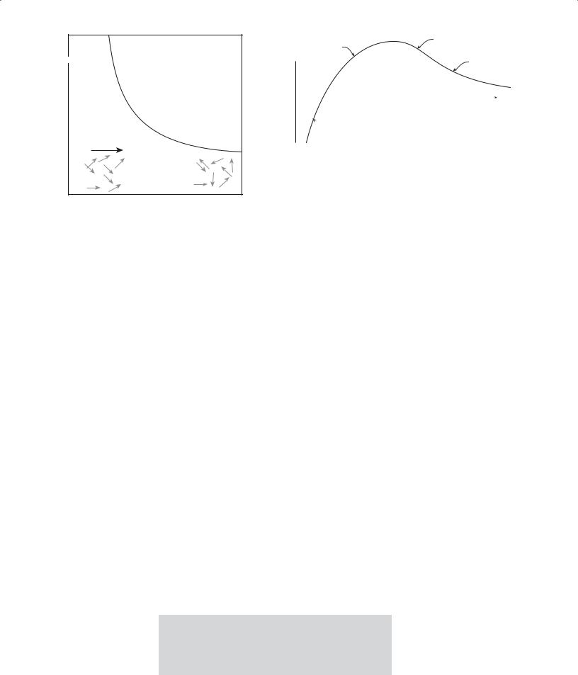
FIGURE 33.5 Schematic showing how χ varies with T for a paramagnetic solid. The insets indicate the direction of the magnetic dipoles in the solids.
energy is more than the energy needed for electron promotion. Some oxides containing transition metal or rare earth ions, such as CeO2 and Cr2O3, are also paramagnetic.
The temperature dependence of paramagnetic susceptibility is shown in Figure 33.5 and follows the Curie law:
χ = |
C |
(33.9) |
|
T |
|||
|
|
There are currently no commercial applications for paramagnetism.
33.8 MEASURING c
The most straightforward way to obtain χ is the classical Gouy method. The material, in the form of a rod, is attached to one arm of a sensitive balance. It is then placed between the poles of a magnet. If the sample is paramagnetic its energy is lower when it is inside the magnetic field, and so there is a force, F, drawing it into the field. If the sample is diamagnetic its energy is less if it is outside the field, and so F is in the opposite direction.
Qualitatively the sign of χ can be determined by whether the force on the sample (the apparent weight change measured by the balance) is positive or negative. We can quantify the value of χ using Eq. 33.10:
F = |
1 |
AχH 2 |
(33.10) |
|
|||
2 |
|
|
|
+ |
|
Fe |
Co |
|
|
|
|
|
|
|
|
||||
|
|
|
|
|
|
||
Exchange |
|
|
|
|
|
||
|
|
|
|
|
|
||
Interaction |
|
|
|
Ni |
|||
0 |
|
|
|
|
|||
|
|
|
|
|
|
|
|
|
|
|
|
|
|
|
|
|
1.5 |
2.0 |
|
|
|
||
|
|
|
D |
||||
|
|
|
|
|
|
||
|
|
|
|
|
|
d |
|
 Mn
Mn
-
FIGURE 33.6 The Slater–Bethe curve showing the magnitude and sign of J as a function of D/d.
the sample by the magnetic field (as in the Gouy method) or on detecting currents induced in a circuit placed close to the magnetic material. The main disadvantage of the Gouy method is that it requires quite a large sample ( grams).
33.9 FERROMAGNETISM
The origin of ferromagnetism, like paramagnetism, is the presence of unpaired electron spins. However, in a ferromagnetic material there is an interaction between adjacent dipoles. Of the first row transition metals only Fe, Co, and Ni are ferromagnetic. So why is Cr paramagnetic not ferromagnetic? The reason is due to a quantum mechanical exchange interaction between the 3d orbitals on adjacent atoms, which is represented mathematically by the exchange integral, J. If J > 0 there is an interaction between adjacent magnetic dipoles causing them to line up and the material is ferromagnetic (below the Curie temperature, θc). If J < 0 adjacent dipoles are antiparallel and the material is antiferromagnetic (below the Néel temperature,
θN).
The magnitude and the size of J depend on the interatomic separation, D, and the diameter, d, of the electron orbital under consideration as shown in Figure 33.6 (the Slater–Bethe curve) for the case of the 3d orbitals of Fe, Co, and Ni.
D can be determined simply by looking up the atomic radius of the element and doubling it, e.g., for Fe r = 0.124 nm and D = 0.248 nm. The value of d can be estimated using Eq. Box 3.2 in Section 3.2. For the 3d orbitals of Fe r = 0.159 nm. Hence D/d is 1.56, as shown in Figure 33.6. J is more difficult to determine. It is related to the overlap of the electron orbitals and involves integrating the products of the wavefunctions for the electron orbitals on adjacent atoms.
where A is the cross-sec- tional area of the sample.
Other methods can be used to determine magnetization and susceptibility, but all rely either on measuring the force exerted on
MEASURING c
It is important to determine χ to know if a material is a superconductor. Having a very low electrical resistivity or an abrupt drop in resistivity is not a defining criterion. A strong magnet has a large value of χ.
If there is significant overlap of the 3d orbitals then, by the requirements of the Pauli exclusion principle, the spins must be antiparallel (J < 0). If the separation is too large then
604 .............................................................................................................. |
U S I N G M A G N E T I C F I E L D S A N D S T O R I N G D A T A |

|
|
|
|
|
|
|
1.0 |
|
|
|
|
|
|
|
|
||
χmag |
|
|
Paramagnetic |
|
|
|
Paramagnetic |
|
|||||||||
|
|
|
|
|
|
|
|
|
|||||||||
|
|
|
|
|
|
|
|
|
|||||||||
|
|
|
|
|
|
|
|
|
|
|
|
|
|
|
|
||
|
|
|
|
|
|
Msat (T) |
|
|
|
|
|
|
|||||
|
|
|
|
|
|
|
|
|
|
|
|
|
|
||||
|
|
|
|
|
|
|
|
Msat (T=0) |
|
|
|
|
|
||||
|
Feromagnetic |
|
|
|
|
|
|
|
|
|
|
Feromagnetic |
|
|
|||
|
|
|
|
|
|
|
|
|
|
|
|
|
|||||
|
|
|
|
|
|
|
|
|
|
|
|
|
|||||
|
|
|
|
|
|
|
|
|
|
|
|
|
|||||
|
|
|
|
|
|
|
|
|
|
|
|
|
|||||
|
|
|
|
|
|
|
|
|
|
|
|
|
|
|
|
|
|
|
|
|
|
|
|
|
|
|
|
|
|
|
|
|
|
|
|
0 |
|
θc |
|
|
|
0 |
|
|
|
T |
|
1.0 |
|||||
|
|
T |
|
|
|
||||||||||||
|
|
|
|
|
θc |
||||||||||||
(A) |
|
|
|
|
|
(B) |
|
|
|
||||||||
|
|
|
|
|
|
|
|
|
|
||||||||
FIGURE 33.7 Schematic showing how (a) χ varies with T;
(b) M varies with T for a ferromagnet.
there is no appreciable interaction. However, in the case of iron, cobalt, and nickel the exchange interaction is large and positive and the electron spins are parallel.
The magnetic susceptibility of a ferromagnetic material varies with temperature (Figure 33.7a) according to the Curie–Weiss law:
χ = C/(T − θc) |
(33.11) |
You will recognize this type of variation as being very similar to an order–disorder transition. Above θc the material become paramagnetic because of randomization of the spin magnetic moments. M decreases from its maximum value at 0 K and vanishes at θc as shown in Figure 33.7(b).
Chromium dioxide (CrO2) is at present the most important ferromagnetic ceramic. It is used as magnetic media in audio and video recording tapes. In this application, the CrO2 is not in the pure form but is usually doped to improve its properties.
CrO2 has the rutile (TiO2) structure (Figure 6.11). The Cr4+ ions are located at the corners of the unit cell and there is a distorted CrO6 octahedron in the center. The lattice parameters are a = 0.437 nm and c = 0.291 nm. CrO2 does not occur in nature and is usually manufactured by thermal decomposition of CrO3 at 500°C under high pressure (>200 MPa) in the presence of water.
33.10 ANTIFERROMAGNETISM AND COLOSSAL MAGNETORESISTANCE
In an antiferromagnet there is exact cancellation of the magnetic moments. We can think of an antiferromagnetic material as consisting of two ferromagnetic lattices in which the spin magnetic moments are equal in magnitude but opposite in direction. Above θN the antiferromagnetic spin alignments are randomized and the material becomes paramagnetic. The temperature dependence of the magnetic susceptibility is shown in Figure 33.8.
The following oxides are antiferromagnetic:
MnO (θN = 122 K) |
NiO (θN = 523 K) |
CoO (θN = 293 K) |
FeO (θN = 198 K) |
χ
Paramagnetic
Antiferromagnetic (antiparallel spins)
|
|
|
θN |
T |
|
FIGURE 33.8 Schematic showing how χ varies with T for an antiferromagnetic material. At θN it becomes paramagnetic.
They all have the rocksalt (NaCl) structure and magnetic dipoles on adjacent {111} planes are antiparallel. The magnetic interaction between the cations occurs indirectly through the oxygen ions and is known as a “superexchange” interaction. Along <100> there is overlap of the Ni dz2 orbitals and the O pz orbital as illustrated in Figure 33.9. The Pauli exclusion principle governs the spin direction in the overlapping orbitals and, as a result, the adjacent Ni ions have opposed spins.
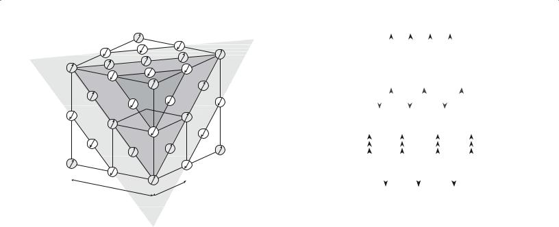
We have direct evidence of the orientation of the spin magnetic moments in antiferromagnetic materials from neutron diffraction studies. Neutrons have a magnetic dipole moment. In neutron diffraction the neutron beam is responding not only to atom positions but also to their magnetic moments. (X-rays give us information on atom positions and electron distribution.) Above θN, the neutron diffraction pattern consists of reflections due to the periodic arrangement of the crystal structure. Below θN extra reflections appear in the pattern because the neutrons are “seeing” two sets of cations, with different magnetic moments. The magnetic unit cell is therefore twice the size of the crystallographic unit cell as shown in Figure 33.10.
Antiferromagnetism is not limited to oxides with a rocksalt structure. The following antiferromagnets have a corundum structure:
V2O3 (θN = 173 K) Ti2O3 (θN = 660 K)
α-Fe2O3 (θN = 950 K)
Although the ceramics we have mentioned so far in this section have no applications that use their magnetic
|
[100] |
|
|
O |
|
Ni |
|
Ni |
dz2 |
pz |
dz2 |
FIGURE 33.9 Overlap between Ni dz2 orbitals and O pz orbitals in Ni.
3 3 .10 A N T I F E R R O M A G N E T I S M A N D C O L O S S A L M A G N E T O R E S I S T A N C E ........................................................................ |
605 |
Ferromagnetic: |
|
|
|
|
|
|
|
|
|
|
|
|
||
|
|
A |
A A |
|||||||||||
|
|
A |
||||||||||||
|
|
B |
|
B |
|
|
|
B |
||||||
Antiferromagnetic: |
|
|
|
|
|
|
|
|
|
|
||||
|
|
|
|
|
|
|
|
|
|
|
|
|||
|
|
|
A |
|
A |
|||||||||
A |
|
|||||||||||||
|
|
|
|
|
|
Ferrimagnetic: |
|
|
|
|
|
|
|
|
|
|
|
|
|
|
|
|
|
|
|
|
|
|
|
|
|
|
|
|
|
|
|
|
|
|
Magnetic unit |
|
Chemical unit |
|
|
|
|
|
|
|
|
|
|
|
|
|
|
||
|
|
|
|
|
|
|
|
|
|
|
|
|
|
|
|
||||
|
|
A B |
A B |
A |
B |
|
A |
||||||||||||
|
|
cell length a |
|
||||||||||||||||
|
cell length 2a |
|
FIGURE 33.11 Schematic comparing dipole alignments in |
||||||||||||||||
|
|
|
|
|
|
||||||||||||||
|
|
|
|
|
|
ferromagnetic, antiferromagnetic, and ferrimagnetic materials. |
|||||||||||||
FIGURE 33.10 Comparison of structural and magnetic unit cells of |
the magnetic moments are not of the same magnitude they |
||||||||||||||||||
NiO. |
|
|
|
|
|
||||||||||||||
|
|
|
|
|
|
only partially cancel each other and the material has a net |
|||||||||||||
|
|
|
|
|
|
M. Ferrimagnetism has several similarities to ferromagne- |
|||||||||||||
properties, |
there |
are manganate ceramics in the |
tism in that the cooperative alignment between magnetic |
||||||||||||||||
La1−xAxMnO3 (0 ≤ x ≤ 1; A = Sr, Ca, Ba) system that are |
dipoles leads to a net magnetic moment even in the absence |
||||||||||||||||||
antiferromagnetic and exhibit colossal magnetoresistance |
of an applied field. Ferrimagnetism is lost above θc. The |
||||||||||||||||||
(CMR). In CMR the resistance drops dramatically in an |
difference between ferromagnetism, antiferromagnetism, |
||||||||||||||||||
applied magnetic field. It is related to, but much greater |
and ferrimagnetism in terms of the spin alignments is |
||||||||||||||||||
than, giant magnetoresistance (GMR) found in multilayers |
illustrated in Figure 33.11. |
|
|
|
|
|
|
|
|
|
|
||||||||
of |
ferromagnetic |
and |
|
|
|
|
|
|
|
The easiest way to con- |
|||||||||
nonferromagnetic |
metals |
|
|
|
|
|
|
sider what happens in a |
|||||||||||
|
ZnFe2O4 |
|
|
||||||||||||||||
(e.g., |
30 Co/Cu bilayers). |
|
|
ferrimagnet is to look at |
|||||||||||||||
In ZnFe2O4 |
[FeIII(ZnIIFeIII)O4] all the magnetic Fe3+ are |
|
|
||||||||||||||||
In these structures there is |
|
the prototypical ferromag- |
|||||||||||||||||
on octahedral sites and are separated by a plane of O2− |
|
|
|||||||||||||||||
an interaction between the |
|
netic |
material, |
magnetite. |
|||||||||||||||
ions. The material is antiferromagnetic because the |
|
|
|||||||||||||||||
ferromagnetic layers that |
|
Magnetite |
|
has |
an |
|
inverse |
||||||||||||
superexchange interaction involving the two Fe3+ ions |
|
|
|
|
|||||||||||||||
can |
cause |
antiferromag- |
|
spinel |
structure |
(Section |
|||||||||||||
resembles that shown in Figure 33.9. |
|
|
|||||||||||||||||
netic ordering of magnetic |
|
7.2). The formula can be |
|||||||||||||||||
|
|
|
|
|
|
||||||||||||||
moments in adjacent layers. |
|
|
|
|
|
|
written as FeIII(FeIIFeIII)O4, |
||||||||||||
So individually each Co layer is ferromagnetic, but the |
i.e., in the classic spinel form AB2O4. The Fe2+ ions and |
||||||||||||||||||
multilayer structure is actually antiferromagnetic. The |
half of the Fe3+ ions are in octahedral sites and the other |
||||||||||||||||||
extent of the interaction depends on the thickness of the |
half of the Fe3+ cations are in tetrahedral sites. The spins |
||||||||||||||||||
nonferromagnetic layer and H. All current hard disk drives |
of the Fe ions on the octahedral sites are parallel, but of |
||||||||||||||||||
make use of this technology. |
|
|
a different magnitude. The spins of the Fe ions on the |
||||||||||||||||
The manganates have the layered perovskite structure |
tetrahedral sites are antiparallel to those in the octahedral |
||||||||||||||||||
similar to that found in the YBCO superconductor (see |
sites. The situation is illustrated in Figure 33.12, which |
||||||||||||||||||
Section 7.16). This similarity is particularly interesting |
shows one-eighth of the magnetite unit cell. The align- |
||||||||||||||||||
and may lead to increased understanding of both types of |
ment of the spins is the result of an exchange interaction |
||||||||||||||||||
material. The nature of the interactions in the manganites |
involving the O2− ions. The antiparallel alignment of the |
||||||||||||||||||
is complicated. They show a metal–insulator transition |
Fe3+ ion in the octahedral site and the Fe3+ ion in the tet- |
||||||||||||||||||
and a ferromagnetic–antiferromagnetic transition associ- |
rahedral site is usually explained by a superexchange reac- |
||||||||||||||||||
ated with CMR. |
|
|
|
tion similar to that used to explain antiferromagnetism. |
|||||||||||||||
|
|
|
|
|
|
A mechanism to account for the parallel spin align- |
|||||||||||||
33.11 FERRIMAGNETISM |
|
ment between the Fe3+ in the octahedral site and the octa- |
|||||||||||||||||
|
hedrally coordinated Fe2+ was proposed by Zener and is |
||||||||||||||||||
|
|
|
|
|
|
called the “double exchange” mechanism. The idea is that |
|||||||||||||
In a ferrimagnet the magnetic moments of one type of ion |
an electron from the Fe2+ ion (3d6) is transferred to the |
||||||||||||||||||
on one type of lattice site in the crystal are aligned anti- |
oxygen in the face-centered position of the subcell shown |
||||||||||||||||||
parallel to those of ions on another lattice site. Because |
in Figure 33.12. At the same time there is transfer of an |
||||||||||||||||||
606 .............................................................................................................. U S I N G M A G N E T I C |
F I E L D S |
A N D |
S T O R I N G D A T A |
||||||||||||||||

Fe3+ (5μB)oct
Fe2+ (4μB)
 O2–
O2–
Fe3+ (5μB)tet
0.419 nm
FIGURE 33.12 Subcell of magnetite showing the location of Fe ions and their spin moments.
electron with parallel spin to the Fe3+ ion. The process is illustrated in Figure 33.13 and shares similarities with the electron-hopping model of conduction in transition metal oxides. (Note: a requirement of Zener’s model is that the cations have different charges.)
Ferrimagnetic ceramics have the spinel (almost exclusively inverse), the garnet, or the magnetoplumbite structure. Table 33.6 lists some examples of ferrimagnetic
Fe2+ (3d6) |
O2– (2p6) |
Fe3+ (3d5) |
||||||||||||||
|
|
|
|
|
|
|
|
|
|
|
|
|
|
|
|
|
|
|
|
|
|
|
|
|
|
|
|
|
|
|
|
|
|
|
|
|
|
|
|
|
|
|
|
|
|
|
|
|
|
|
|
|
|
|
|
|
|
|
|
|
|
|
|
|
|
|
|
|
|
|
|
|
|
|
|
|
|
|
|
|
|
|
|
|
|
|
|
|
|
|
|
|
|
|
|
|
|
|
|
|
|
Before |
|
|
Fe3+ (3d5) |
O1– (2p5) |
Fe2+ (3d6) |
After |
|
|
FIGURE 33.13 Illustration of the double exchange interaction in |
||
magnetite. |
|
|
spinels and their properties. The magnetic moments in this table were calculated taking account of only the number of unpaired 3d electrons; the units are Bohr magnetons and the minus sign denotes an antiferromagnetic coupling.
The most important and widely studied magnetic garnet is yttrium–iron garnet (YIG), which has the formula Y3Fe2(FeO4)3 [remember garnet is Ca3Al2(SiO4)3]. We can write the formula of YIG as Y3c Fea2 Fed3O12 where the superscripts refer to the type of lattice site occupied by each cation. The cell shown in Figure 33.14 is actually one of the eight subcells that form the YIG unit cell, which contains 160 atoms. In the subcell the a ions are in a body-centered cubic (bcc) type arrangement with the
TABLE 33.6 Magnetic Properties of Several Ferrimagnetic Ceramics
|
|
Bsat (T) |
Calculated moments |
|
|
||
|
qc (K) |
|
|
|
|
|
|
|
|
|
|
|
|
||
Material |
at RT |
T site |
O site |
Net |
Experimental |
||
|
|
|
|
|
|
|
|
Fe3+ [Cu2+ Fe3+]O4 |
Spinel ferrites [AO · B2O3] |
−5 |
|
+ 5 |
|
|
|
728 |
0.20 |
1.73 |
1 |
1.30 |
|||
Fe3+ [Ni2+ Fe3+]O4 |
858 |
0.34 |
−5 |
2 |
+ 5 |
2 |
2.40 |
Fe3+ [Co2+ Fe3+]O4 |
1020 |
0.50 |
−5 |
3 |
+ 5 |
3 |
3.70–3.90 |
Fe3+ [Fe2+ Fe3+]O4 |
858 |
0.60 |
−5 |
4 |
+ 5 |
4 |
4.10 |
Fe3+ [Mn2+ Fe3+]O4 |
573 |
0.51 |
−5 |
5 |
+ 5 |
5 |
4.60–5.0 |
Fe3+ [Lio.5Fe1.5]O4 |
943 |
|
−5 |
0 |
+ 0.75 |
|
2.60 |
Mg0.1Fe0.9[Mg0.9Fe1.1]O4 |
713 |
0.14 |
0–4.5 |
0 |
+ 5.5 |
1 |
1.10 |
|
Hexagonal ferrites |
|
|
|
|
|
|
BaO : 6Fe2O3 |
723 |
0.48 |
|
|
|
|
1.10 |
SrO : 6Fe2O3 |
723 |
0.48 |
|
|
|
|
1.10 |
Y2O3 : 5Fe2O3 |
560 |
0.16 |
|
|
|
|
5.00 |
BaO : 9Fe2O3 |
718 |
0.65 |
|
|
|
|
|
|
|
Garnets |
|
|
|
|
|
YIG{Y3}[Fe2]Fe3O12 |
560 |
0.16 |
|
|
|
5 |
4.96 |
(Gd3)[Fe2]Fe3O12 |
560 |
|
|
|
|
16 |
15.20 |
|
|
Binary oxides |
|
|
|
|
|
EuO |
69 |
|
|
|
|
|
6.8 |
CrO2 |
386 |
0.49 |
|
|
|
|
2.00 |
|
|
|
|
|
|
|
|
3 3 .11 F E R R I M A G N E T I S M ................................................................................................................................................... |
607 |