Symbolic calculations.

You’ve seen Mathcad engaging in numeric calculations. This means that whenever you evaluate an expression, Mathcad returns one or more numbers, as shown at the top of Figure 14-1. When Mathcad engages in symbolic mathematics, however, the result of evaluating an expression is generally another expression, as shown in the bottom of Figure 14-1.

Figure 14-1: A numeric and symbolic evaluation of the same expression.

Example 1: Factoring and expanding expressions

Enter an expression. Press the space bar until the entire expression is boxed.

Select Symbolics - Expand or Symbolics - Factor to expand or factor the expression.

Boxing (x 1).(x 4) and then selecting Symbolics - Expand yields: x2 5.x 4

Boxing x2 5.x 4 and then selecting Symbolics - Factor yields: (x 1).(x 4)

Example 2: Evaluating symbolic expressions

Two method is illustrated below:

1) Using Symbolics - Evaluate - Symbolically from the main menu

and then selecting Symbolics - Evaluate - Symbolically yields:

Example 3: Simplyfing symbolic expressions

Enter an expression. Press the space bar until the entire expression is boxed.

Select Symbolics - Simplify.

Example 4: Solving symbolic equations using a SOLVE BLOCK

There are two main differences from a regular Solve Block:

1) Do not use initial guesses.

2) Use the symbolic evaluation operator (right arrow) with the Find function.

The order of the work performance

Task 1.

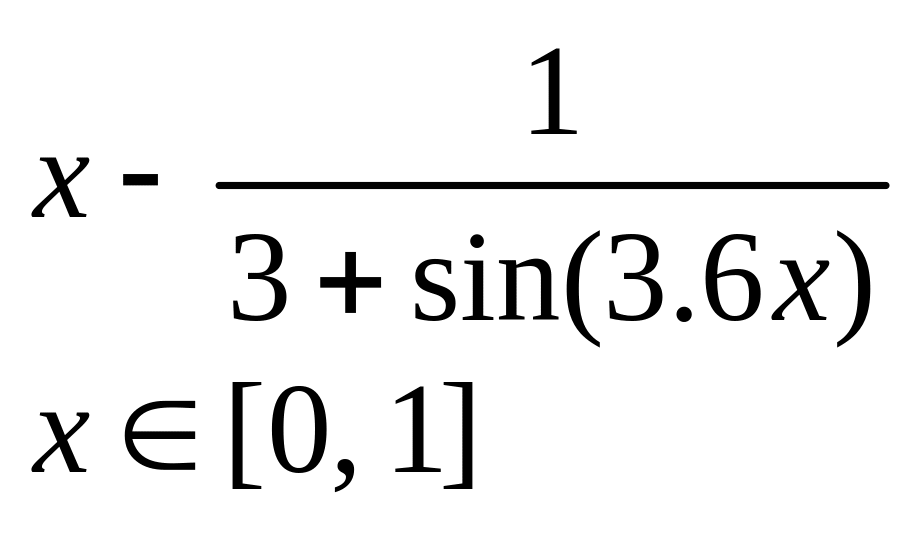
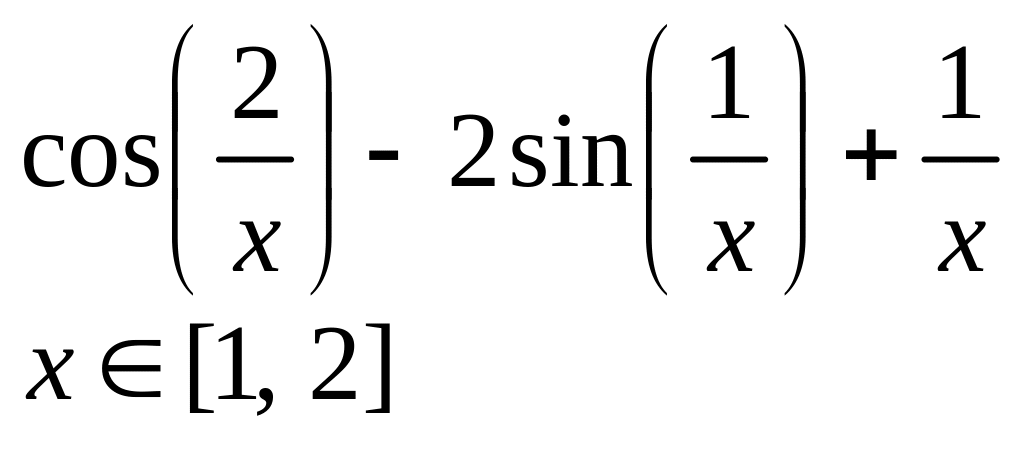
Create the graph of the function f (x) (Table 1) and determine one of the roots of the equation approximately. Solve the equation f (x) = 0 with a built-in Mathcad root function up to the accuracy equals  = 10 ^{– 4};

Table 1

Variants

Variant	f(x)	Variant	f(x)
			arccos -x х  2, 3]
			х5 – х - 0,2 х  1, 2]

Task 2.

For a polynomial g (x) (Table 2) perform the following:

1) using the command symbols  coefficients create the vector V, which contains the polynomial coefficients;

2) solve the equation g (x) = 0 using the polyroots;

3) solve the equation symbolically.

Table 2

Variants 2

Variant	g(x)	Variant	g(x)
	x4 - 2x3 + x2 - 12x + 20		x4 + x3 - 17x2 - 45x - 100
	x4 + 6x3 + x2 - 4x - 60		x4 - 5x3 + x2 - 15x + 50
	x4 - 14x2 - 40x - 75		x4 - 4x3 - 2x2 - 20x + 25
	x4 - x3 + x2 - 11x + 10		x4 + 5x3 + 7x2 + 7x - 20
	x4 - x3 - 29x2 - 71x -140		x4 - 7x3 + 7x2 - 5x + 100
	x4 + 7x3 + 9x2 + 13x - 30		x4 + 10x3 +36x2 +70x+ 75
	x4 + 3x3 - 23x2 - 55x - 150		x4 + 9x3 + 31x2 + 59x+ 60
	x4 - 6x3 + 4x2 + 10x + 75

Task 3.

Solve the system of linear equations (Table 3):

1) using the Find;

2) using the matrix method and the lsolve.

Table 3

Variants 3

Variant	system of linear equations	Variant	system of linear equations

Task 4.

Преобразовать нелинейные уравнения системы из Таблицы 4 к виду f ₁(x) = y и f ₂ (y)= x. Построить их графики и определить начальное приближение решения.  Решить систему нелинейных уравнений с помощью функции Minerr.

Convert non-linear equation system in Table 4 in the form f ₁(x) = y and f ₂ (y)= x. Build their graphs and determine the initial approximation of the solution. Solve the system of nonlinear equations using the Minerr.

Table 4