Hi!

Thanks for buying Welsh’s Synthesizer Cookbook! You’ll find that the approach of this book is different than other synthesizer books you may have read. The two most important differences between this book and others are the universal patches and the heavy emphasis on harmonics. The patches were written because after years of searching I found that there was no other patch book that could be used on all dual-oscillator analog/subtractive synths. Sure there are copies of 70s era patch books around, but they are specific to particular models and of limited use with other equipment. In the many decades that analog synthesis has been around no one, to the best of my knowledge, ever created a general-purpose patch book. Definitely not one where the acoustic emulations are based on the harmonics of the actual instruments!

When I first started creating the patches for the book back in late 2004 I was not yet using harmonic analysis. The sounds were being created the old fashioned way; by ear. That’s how I’d been making sound for the past decade, and I had no problem with it.

Sure I’d heard of harmonic analysis. It was that thing that synth books would sometimes make a passing reference to or they might even dedicate an entire paragraph about it. It was that “neat looking but mostly unused” graphic that could be activated in most sound editors. Well, partway into creating the Cookbook patches I had one of those paradigm- shifting moments that happens to every synth player once every few years. It occurred to me that a harmonic analyzer might be useful for analyzing and recreating acoustic instruments. That’s when I discovered MDSPs Fre(a)koscope VST plugin and everything changed in an instant. With a bit of practice this tool granted a higher level of control and precision to my sound sculpting that I would not have thought possible. This is not referring solely to recreating acoustic instruments either. Sounds from other analog synths are absolute cake to pick apart. Harmonic analysis makes analog programming much more powerful and it even makes FM synthesis substantially easier.

The earlier patches were redone and subsequent patches were created using the harmonic analysis. As more and more patches were created using the analyzer it became apparent that the most useful piece of knowledge that I could impart to anyone was the use of harmonic analysis for analyzing sounds as well as a means for understanding the behavior of each parameter on a synth. I’ve used harmonic analysis to recreate my own voice on an analog synth, recreate an acoustic piano which is generally considered impossible, and even duplicate sounds used in songs without sampling! One of the goals of this book is to give the reader this same ability. Thanks again and enjoy using the Synthesizer Cookbook!

Regards.

Fred Welsh

PATCH QUICK START: The filter cutoff frequency is the one parameter where getting the correct setting is most critical. If your synthesizer's filter doesn't give cutoff frequency values in Hz/kHz and the percentage values in the book don't seem to produce the correct results and if you don’t feel like going through the whole calibration routine at the back of the book then to get off to a quick start do the following: Set the synth to output a single sawtooth. Set the filter’s cutoff frequency to the very middle of its range and match the output to one of the sound files on the CD in the Calibration Sound Files Filter -> 12 db or 24 db subfolder. The name of the sound file that matches the output gives the approximate cutoff frequency (in FIz) that corresponds to the middle position. Assume the lowest dial position of your synth’s cutoff frequency is 20 Hz and the highest position is a cutoff frequency of 20,000 Hz (20 kHz). These two values may not be correct for your synth but they will be close enough sound wise. Knowing just these three values, low, mid, and high, will actually make approximating the filter cutoff settings listed in the patches quite a bit more accurate.

Note: filter cutoff frequency settings generally do not operate on a linear scale so if you come up with a middle setting of something like 300 Hz, 600 Hz, 1200 Hz etc. i: is probably correct. In other words, the mid value is not going to be anywhere near 10.010 Hz which would be the numerical mid point between 20 Hz and 20,000 Hz.

Also be sure to check out: “Tri-Osc” t-shirt $12.95

Shirt features the Synthesizer Cookbook triple oscillator logo across the front. Yellow print on a black 100% cotton t-shirt. For more details, be sure to visit: www.synthesizer-cookbook.com

Contents

OSCILLATORS	1	SYNTHESIS THROUGH HARMONIC ANALYSIS AND
Harmonics & waveforms	1	REVERSE ENGINEERING	29
Pulse width	7	Reverse engineering a a patch from another
Syncing	9	synth	30
Noise Keyboard tracking	12 13	Reverse engineering a sound from a song Emulating an acoustic	34
Polyphony Portamento	14 14	instrument’s harmonics and envelope: clarinet	39
Unison	14	COOKBOOK PATCHES	47
Ring modulation	15	Instructions	47
FILTERS	16	String patches	53
Filter types	16	Woodwinds	63
Cutoff frequency	18	Brass	69
Filter slope	18	Keyboards	73
Resonance	20	Vocals	77
ENVELOPES	22	Tuned percussion	81
LFOs	24	Untuned percussion	85
Pulse-width modulation	25	Leads	91
Beat effects	26	Bass	95
Sample & hold	27	Pads	99
Sync sweeping	27	Sound Effects	105
KEYBOARD EXPRESSION	27	CALIBRATION	111
Velocity sensitivity	27	Using the CD	111
Aftertouch	27	Using sound editors, meters	115

Patches

STRINGS		KEYBOARDS		New Age Lead 92
Banjo	53	Accordion	73	R&B Slide 93
Cello	53	Celeste	73	Screaming Sync 93
Double Bass	54	Clavichord	74	Strings PWM 94
Dulcimer	54	Electric Piano	74	Trance 5th 94
Guitar, Acoustic	55	Harpsichord	75
Guitar, Electric	55	Organ	75	BASS
Harp	56	Piano	76	Acid Bass 95
Hurdy Gurdy	56			Bass of the Time Lords 95
Kora	57	VOICE		Detroit Bass 96
Lute	57	Angels	77	Deutsche Bass 96
Mandocello	58	Choir	77	Digital Bass 97
Mandolin	58	Vocal, female	78	Funk Bass 97
Riti	59	Vocal, male	78	Growling Bass 98
Sitar	59	Whistling	79	Rez Bass 98
Standup Bass	60
Viola	60	PERCUSSION.	TUNED	PADS
Violin	61	Bell	81	Android Dreams 99
		Bongos	81	Aurora 99
WOODWINDS		Conga	82	Celestial Wash 100
Bagpipes	63	Glockenspiel	82	Dark City 100
Bass Clarinet	63	Marimba	83	Galactic Cathedral 101
Bassoon	64	Timpani	83	Galactic Chapel 101
Clarinet	64	Xylophone	84	Portus 102
Conch Shell	65			Post-Apocalyptic
Contrabassoon	65	PERCUSSION.	UNTUNED	Sync Sweep 102
Didgeridoo	66	Bass Drum	85	Terra Enceladus 103
English Horn	66	Castanets	85
Flute	67	Clap	86	SOUND EFFECTS
Oboe	67	Claves	86	Cat 105
Piccolo	68	Cowbell	87	Digital Alarm Clock 105
		Cowbell, analog	87	Journey to the Core 106
BRASS		Cymbal	88	Kazoo 106
French Horn	69	Side Stick	88	Laser 107
Harmonica	69	Snare Drum	89	Motor 107
Penny Whistle	70	Tambourine	89	Nerd-O-Tron 2000 108
Saxophone	70	Wheels of Steel	90	Ocean Waves
Trombone	71			(with fog horn) 108
Trumpet	71	LEADS		Positronic Rhythm 109
Tuba	72	Brass Section	91	Space Attack! 109
		Mellow 70s Lead 91		Toad 110
		Mono Solo	92	Wind 110

Harmonics and oscillator waveforms

The most fundamental sound is the sine wave. Every sound whether it is natural or synthetic is made up of sine waves.

Figure 1. All sounds, natural and synthetic, are made up of sine waves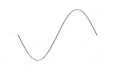

The sound of a sine wave could be described as extremely mellow and not particularly interesting, but when numerous sine waves of different pitches and amplitudes are mixed together the sonic possibilities become endless.

440 Hz Sine

It is possible to create any waveform using nothing but sine waves. Let’s begin by creating a sawtooth wave. Each sine wave is going to have a different pitch and as they go higher in pitch they will decrease in amplitude. The first one will have the lowest pitch and it will in fact determine the overall pitch of the sawtooth. This is called the fundamental frequency. For the case of this example we will give it a pitch of 440 Hz corresponding to the A4 key.

Figure 2. A 440 Hz sine wave and a graph representing its frequency and amplitude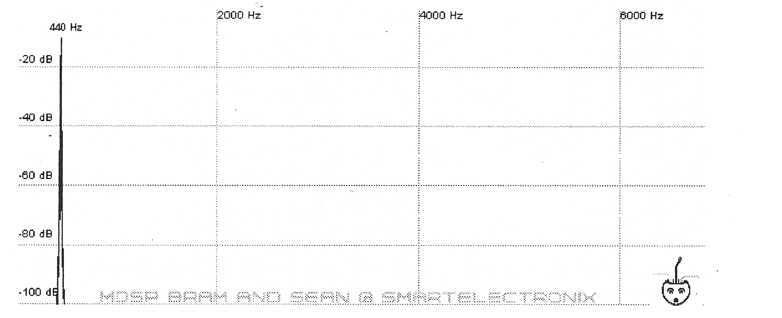

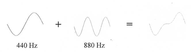The bottom portion of the figure is what is called a harmonic diagram. The horizontal axis is frequency/pitch and the vertical axis is amplitude. The spike represents the frequency and amplitude of the 440 sine wave. Let’s add a second sine wave with a frequency of 880 Hz (440Hz x 2).

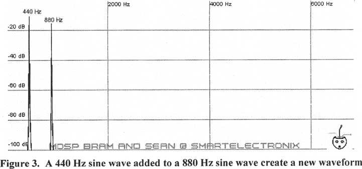
Notice there is a second spike in the diagram representing the 880 Hz sine wave. Now add a third sine wave at a frequency of 1320 Hz (440 Hz x 3)

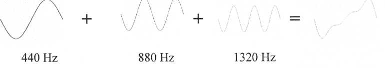
Figure 4. Three sine waves of frequency 440 Hz, 880 Hz, and 1320 Hz added together create a waveform that begins to look like a sawtooth wave.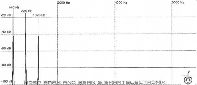

Already the new waveform is beginning to lean to one side like a sawtooth wave. Keep adding sine waves that are frequency multiples of 440 Hz and eventually a sawtooth wave is produced.

Figure 5. A sawtooth wave and its harmonic diagram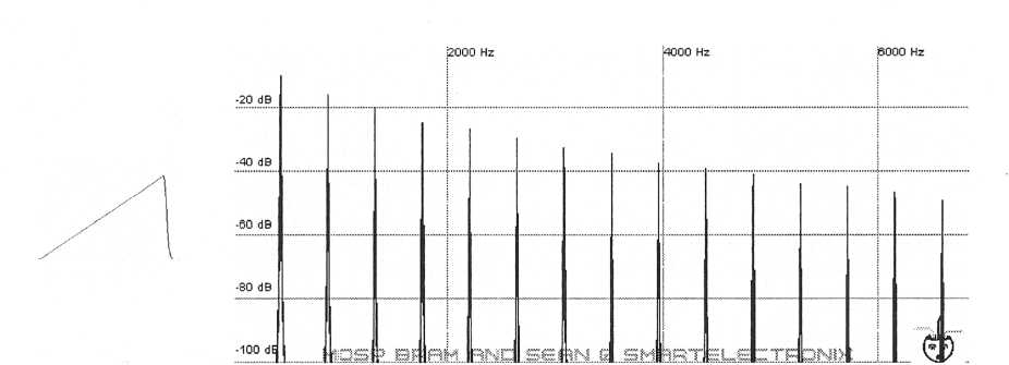

Each one of the harmonics(spikes) in the diagrams above are called partials. The first partial at the far left, as stated earlier, is known as the fundamental and it determines the pitch of the waveform. The other partials are all frequency multiples of the fundamental and they are known as overtones. Also notice that the fundamental is the loudest sine wave of all the harmonics and that as the overtones get higher in pitch their amplitudes decrease. There is of course nothing preventing us from mixing sine waves that all have the same amplitude it’s just that in this particular case it is a requirement of creating a sawtooth that the amplitudes diminish with higher frequency. Just as a point of interest if we were to mix these harmonics all at the same amplitude it would produce something that as successively higher-pitched sine waves are added would at first look like a sawtooth wave with a bad complexion and as more harmonics are added would look nothing like a sawtooth at all. Harmonic amplitudes are important!

Figure 6. Waveform produced by setting the first 16 harmonics to equal amplitudes.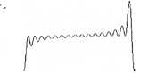

A square wave can be created using the same process. The difference is that a square wave is only made up of odd-numbered partials.

Figure 7. A square wave has only odd partials. This square wave was produced by an actual oscillator. Notice the slight imperfections in the waveform. No oscillator produces perfect waveforms nor do any two oscillators produce identical waveforms.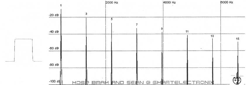

Triangle waves are also made up of odd-numbered partials but the higher harmonics are weaker than in a square wave.

Figure 8. A triangle wave has odd harmonics that are weaker than those of a square wave.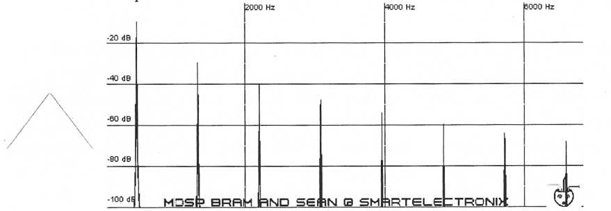

The process of adding sine waves together to create sounds is known as additive synthesis. This method is used on a few digital synthesizers and soft synths and has also been used by pipe organs for hundreds of years. In a pipe organ each pipe produces a sine wave of a different pitch and by controlling the amount of air to each pipe it is possible to control the individual amplitudes of each sine wave which in turn makes it possible to produce sounds that are harmonically similar to other instruments. It could be said that pipe organs were the first synthesizers.

Analog synthesizers use a process called subtractive synthesis which is simply additive synthesis in reverse. Here’s some synth terminology for you: Sounds created by synthesizers are referred to as patches. This goes back to the early days of modular synthesizers when patch cables were used to route signals from module to module to

create a sound. Patches created using subtractive synthesis start with waveforms that are already rich in harmonics such as sawtooth, square, and triangle waves. These waveforms are then passed to a filter which removes harmonics from the waveforms in order to produce the desired sound. The harmonics are subtracted out hence the process is known as subtractive synthesis.

The most common waveforms on analog synthesizers are the sawtooth, square/pulse, and triangle wave. There are three main reasons these are used almost universally rather than other waveforms. First is the fact that they all have lots of harmonics which can be chiseled away by the filter. Secondly they are relatively easy to produce using analog circuits. Thirdly they are each harmonically similar to broad families of acoustic sounds even without any filtering. This almost sounds as if to imply that acoustic imitation is the goal of synthesis which it most certainly is not. It is a practical criteria to start with if nothing else. Sawtooth waves are similar to brass and string instruments, square waves are similar to woodwinds, and triangle waves with their diminished higher harmonics are good for mixing together to produce inharmonic sounds (bells, chimes, etc) as well as adding the occasional rogue harmonic to saw and pulse waveforms. This may be surprising but even though these waveforms have similar harmonics and sound similar to certain families of instruments the waveforms of acoustic instruments look nothing like squares/pulses, sawtooths, or triangles. A waveform’s usefulness lies with the harmonics that make it up and is NOT inherent to the shape of the waveform. Two sounds can have very similar harmonics yet have waveforms that look nothing alike. Adding waveforms together in an attempt to match the waveshape of an acoustic instrument won’t produce desirable results most of the time.

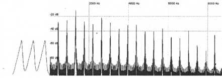
While some synthesizers only have one oscillator and a few others have many, the majority have two oscillators that can be independently set to different waveforms. Two- oscillator configurations are so common because they are cheaper to produce than multi- oscillator synths yet they are much more capable of producing rich sounds than single- oscillator instruments. They are a good balance of economy and ability. By using two oscillators it is possible to not only create more interesting strings, brass, and woodwinds but it also becomes possible to create vocals, inharmonic sounds such as bells, and countless other acoustic and synthetic sounds. One simple fact is that a single oscillator will have harmonics where each successive partial has less amplitude. While the higher harmonics of acoustic instruments do diminish in amplitude they do not follow this progression so rigidly. Below are harmonic diagrams of some acoustic instruments.

Figure 9. Violin harmonics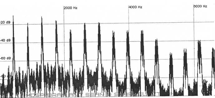

Figure 10. Flute harmonics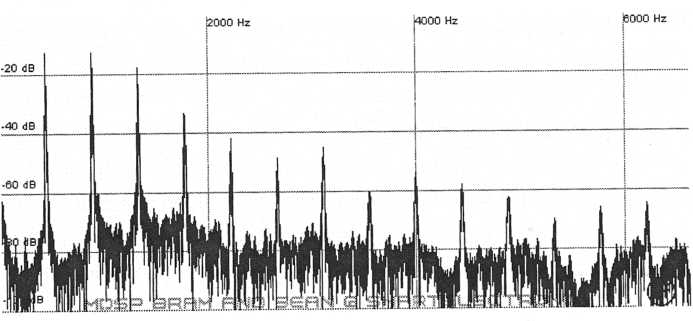

The noise at the bottom of the graphs is from resonance, reverberation, and recording noise.

Notice that while the higher harmonics do die away they do not do so in a uniform fashion like synthetic waveforms. These slight harmonic deviations help separate one acoustic instrument from another in the same family and give what could be considered a “natural” sound. Again, imitation is a possibility of synthesis but is not necessarily the goal, however lessons learned from studying and recreating acoustic sounds can help to produce more interesting synthetic patches that have character and life. By detuning oscillators it is possible to come up with much more interesting sounds. To produce the harmonics of a marimba for example take a triangle wave and add a second triangle wave at slightly lower amplitude and tuned up two octaves.

Figure 12. Using two oscillators to synthesize an instrument such as the marimba allows for a more complex harmonic structure than using single waveforms alone.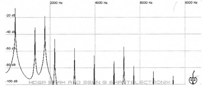

By simply mixing two humble triangle waves with different tunings a more harmonically sophisticated sound has been produced than could be done with just a single waveform. The harmonics of a single triangle may die out uniformly but the harmonics of two detuned triangles do not. While this sound is literally the sum of two triangle waves, to the ear it sounds far richer than the sum of its parts. The important point here is that using two oscillators gives more control over the harmonic make up of the final sound. As we shall see there are many other tools at our disposal that will allow us to further fine tune harmonic structure.

Pulse-width

A feature available on most analog synths is the ability to use a variable-width pulse as a sound source. Square waves are actually a form of pulse. A square wave is a pulse with a width of 50% since the pulse is active for half of the wave cycle. By changing the width of a pulse it is possible to change its harmonic content.

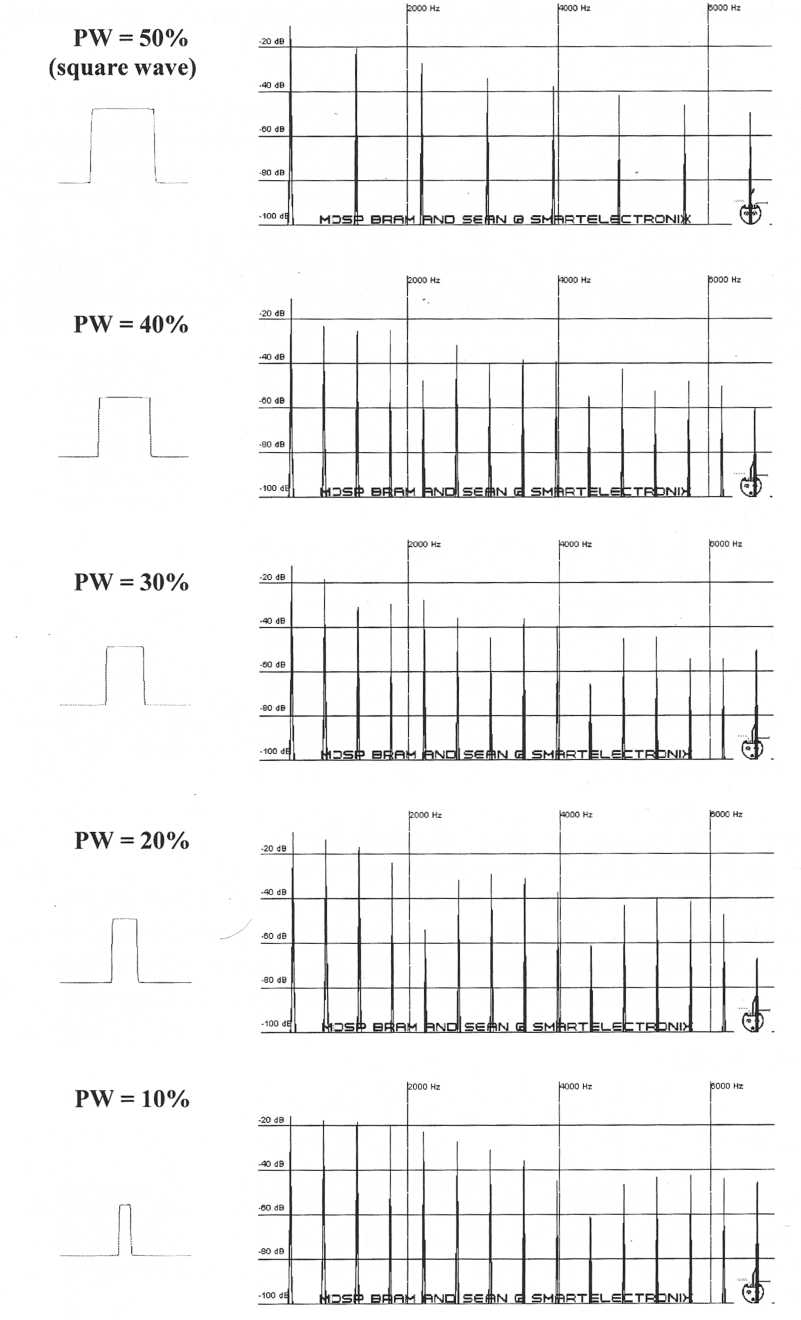
Figure 13. Pulse widths. Narrowing the pulse width creates a brighter, edgier sound similar to a sawtooth.

As a pulse becomes narrower it goes from a square wave with only odd partials to having both even and odd partials and therefore sounding more like a sawtooth wave. Look at the figures above and you’ll notice that even though narrow pulses have harmonic spectra that are similar to a sawtooth there are still some important differences. The harmonics do not die out as quickly or with the same uniformity as those of a sawtooth. Narrow pulses have more of a crisp, metallic sound. By narrowing the pulse width it is also possible to give the harmonics an “undulating” pattern similar to the harmonic behavior of many acoustic instruments. The advantage of a pulse with variable width is that it allows a higher degree of control over the harmonics than using just waveform mixing and filtering alone. Another cool thing about variable-width pulses is that the width can usually be modulated to produce thick string-like patches. More about that in the section on LFOs. Some synths don’t provide the ability to change the width of the pulse, but these instruments often provide a few pulses that are hardwired to different widths. This is common on ROMpler, sample-based instruments and even a few analog synths.

Syncing

Another common feature with most dual-oscillator analog synths is the ability to sync one oscillator to the other. This is useful for producing, amongst other things, plucked and hammered strings such as pianos and guitars. Syncing forces the wavecycle of one oscillator to restart when the wavecycle of the other oscillator restarts. The oscillator that is being synced is called the slave while the oscillator it is synced to is called the master. Usually, but not always, a synthesizer’s second oscillator is the slave while oscillator one is the master. You may want to check your synth’s manual to be sure since it’s often not clear on the front panel. For syncing to have any effect on the sound the synced oscillator must be tuned higher than the master oscillator.

When the slave oscillator is tuned higher than the master oscillator its waveform will restart each time the waveform of the master restarts. The resulting waveform produced by the slave using a sawtooth would look similar to that shown at the bottom of the following figure. When synced, the tuning of the master also controls the actual tuning of the slave while any changes that are made using the slave’s tuning/pitch control will instead change the tonal qualities of the oscillator.

SLAVE

UNSYNCED

SLAVE’S

SYNCED

OUTPUT

MASTER

Figure 14. When a slave oscillator is synced its waveform will restart every time the master oscillator restarts.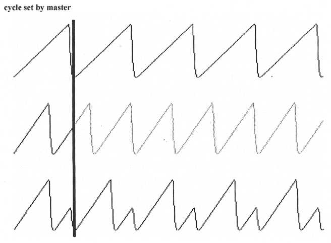

Here’s an example that you may want to try for yourself. Start by setting the slave oscillator to produce a sawtooth waveform. The waveform used by the master doesn’t matter. Only its pitch matters since it controls the wave cycle time. Turn the volume of the master oscillator all the way down but make sure it is turned on. We want the master to be available for syncing the slave but we don’t want to hear the master’s output. Set both oscillators to the same pitch. If you now turn syncing on and off you will notice that the output of the slave sounds the same either way. This is because the master is making the slave’s waveform restart at the same location that it would even if the two weren’t synced since the pitch settings are identical.

Next turn syncing on and slowly increase the pitch of the slave without going as high as one octave above the pitch set by the master. As it increases the output of the slave will take on a thin, brittle timbre, however the overall pitch stays the same.

Turn the slave’s pitch control up to the point where it corresponds to exactly one octave higher than the pitch setting of the master. If we now turn syncing off we will hear no change. The brittle timbre is gone and you are now hearing a plain sawtooth only it is an octave higher in pitch. Even though the slave is indeed tuned higher than the master it’s pitch is now exactly double that of the master and therefore the master is causing the slave to once again restart at a point where it would restart even if it weren’t synced. A further increase of the slave’s pitch will continue to produce metallic, harmonically-rich sound until the slave is pitched two octaves above the master, and so on. To summarize: The slave must be tuned higher but if it is tuned at octave intervals syncing will have no effect. Look at the figures below. As the slave’s pitch setting is increased the harmonics change, but when the slave’s pitch is set to one octave above the master the output simply becomes that of a plain sawtooth (or square) tuned one octave higher in pitch.

SYNCED SAWTOOTH SYNCED SQUARE

SYNCED SQUARE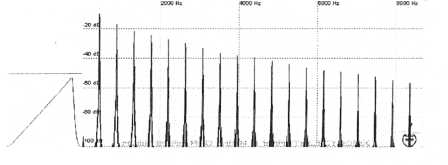

Slave’s pitch = Master’s pitch

Slave = Master + 4 semitones

Slave = Master + 8 semitones

Slave = Master +12 semitones (I octave)

Slave = Master +16 semitones

Slave = Master + 20 semitones

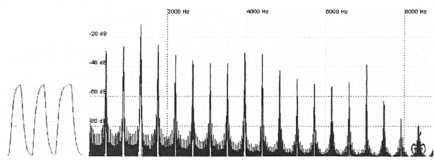
Figure 15. Harmonics of synced sawtooth and square waveforms are much more complex than unsynced waveforms. Detuning the slave from the master by octave intervals negates the syncing effect since the slave is forced to restart at a location where it would restart even if it weren’t synced.

Noise

There is pink noise which diminishes in power by 3 dB per octave.

Subtractive synthesizers generally have two types of sound sources. One of these sources are the oscillators while another is noise. On some models the noise source is actually provided by one of the oscillators while on others it is provided separately. Noise is useful for creating many percussion sounds, creating sound effects such as ocean waves and wind, and driving filter resonance. The most common form is white noise which maintains uniform power across all frequencies. Television static is white noise.

Figure 16. White noise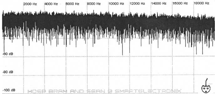

Figure 17. Pink noise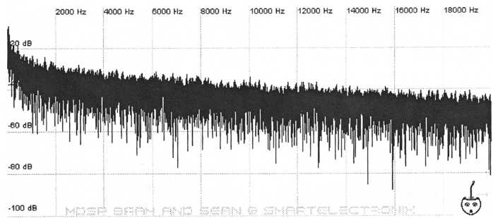

There is also brown noise which diminishes in power by 6 dB per octave. Put simply, white noise sounds brighter than pink noise, and pink noise sounds brighter than brown.

Figure 18. Brown noise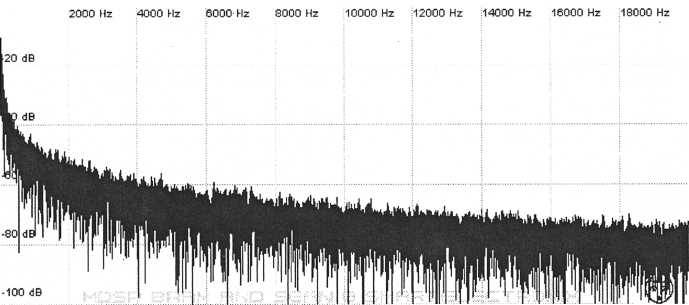

What distinguishes noise from a typical waveform is that it has no harmonic partials and the sound is spread solidly across the audio spectrum. True noise has no pitch. When noise is used to create percussive patches such as snare drums or cymbals it may use filter resonance or sometimes a triangle wave will be mixed in to impart a sense of pitch.

With a regular oscillator waveform pitch, pulse width, and syncing can all be controlled to manipulate the sound before it reaches the filter. Noise has none of these controls and therefore is highly dependent upon the filter for sculpting. Noise when used along with the filter, and the filter’s resonance and envelope is far more useful than it may at first seem.

Keyboard Tracking

Oscillator keyboard tracking, sometimes called keyboard pitch tracking, allows the user to select whether or not the pitch of an oscillator will change as different keys are played. Turning this off will cause the same pitch to be sounded by every key. This can be particularly useful when creating bagpipes, sitars, and other drone instruments. Bagpipes and sitars are similar in the respect that they both play a set of notes of varying pitch over top a drone of unchanging pitch. Use one oscillator with tracking turned on to play the notes of varying pitch and use a second oscillator with tracking turned off to imitate the drone. The pitch control sets the single pitch that is played on all keys. It is quite common for an untracked oscillator pitch to correspond with the same pitch that would be played by either the C4 or A4 keys if tracking were turned on.

Keyboard tracking is sometimes offered as a control on other parameters as well in addition to pitch. After pitch tracking, the most common is filter cutoff keyboard tracking. This can be used to either gradually increase or decrease the amount of filtering that takes place as keys are played either up or down the keyboard. For example, if the high notes in a patch sound too bright keyboard tracking can be used to give them more filtering while letting the lower notes pass through unfiltered. Keyboard tracking is also occasionally used to modify envelope times and amounts. It can be used to give higher notes faster envelope times which can be useful for creating piano patches where high notes decay faster than lower ones.

Polyphony

Polyphony refers to the number of keys that can be played and still produce sound. For example, a synthesizer with five-note polyphony will produce sound for a maximum of five notes at a time. What would happen if more than five keys were played? This depends on the synthesizer. Some synths will “steal” notes that have been held the longest in order to play newer notes while other synths may steal the lowest-pitched, or highest-pitched notes. Many synths allow the user to choose the method of note stealing that they prefer.

Synthesizers that only allow one note to be played at a time are called monophonic while synthesizers that allow multiple notes are polyphonic. Most early synthesizers were strictly monophonic. Monophonic playing isn’t always a limitation. In fact most modern synths give the user the option to choose between monophonic and polyphonic playing. Monophonic playing can be particularly useful for some leads and bass patches. It helps to keep a single patch from over-dominating a mix and sounds particularly interesting when used in conjunction with portamento.

Portamento

Portamento, also known as glide, will cause the pitch to change gradually between two consecutively struck keys. This is controlled by a time parameter which determines how long it takes for the pitch to change. There is often a setting that will determine whether glide is only present when the keys are played overlapping (legato) or glide is automatic whether the keys overlap or not.

Unison

Unison is used to create a chorusing-like effect. Historically this has been achieved by using all of a polyphonic synth’s oscillators to play the same note and would effectively make the instrument monophonic when in unison mode. The fact that true analog oscillators cannot keep exactly the same tuning becomes an asset here. Because all of the oscillators are slightly detuned from each other over the range of a few cents the sound is very thick. The sound is also somewhat similar to that produced by pulse-width modulation. The graph below shows a sawtooth wave being played in unison. The higher harmonics are broadened similar to the way they would be in pulse-width modulation. Unison unlike PWM, as we will discuss later, doesn’t flatten out the harmonic levels and it also adds some low-amplitude, inharmonic content. Notice how the harmonics are broadened similar to those of the violin graph at the top of page 6. Unison is often used to create bowed-string sounds.

Figure 19. Unison broadens the harmonics of a waveform creating a chorus- like effect.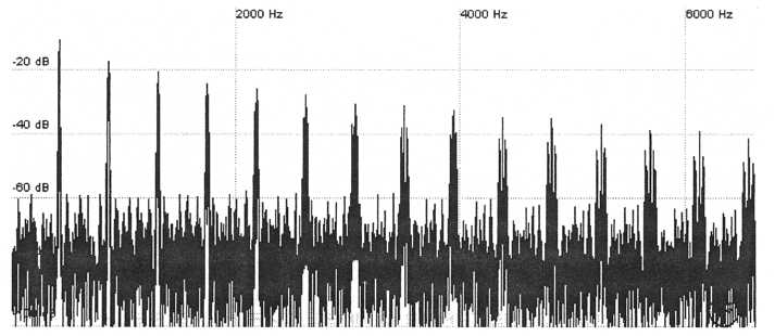

Unison is also particularly good for use with filtered pads as well as beastly, bone- crunching leads. If your synth allows you to set the amount of unison try decreasing it to keep it from becoming too overbearing. Except of course when you want it to sound beastly!

Ring Modulation

Even though the synthesizer provided with this book and the included patches do not use ring modulation it is nonetheless common enough that it deserves some explanation.

Ring modulation works by multiplying two signals together which produces an output that consists of frequencies that are the sum and difference of all the original harmonic frequencies. For example take two harmonics which each belong to separate signal inputs on a ring modulator. If one has a frequency of 50 hz and the other has a frequency of 150 hz then the signal put out by the ring modulator will have harmonics at 100 hz and 200 hz. This particular example illustrates the process but it may not seem to be particularly useful since we are just taking two harmonics and producing two different harmonics. The important point to consider is that in practical usage every harmonic in one signal gets multiplied with every harmonic in the other. If the two signals have tunings where many of their harmonics coincide then the end result will be a harmonic sound with rich overtones.

If the oscillators are set to inharmonic intervals the ring modulator will produce a rich inharmonic sound that is harsh and metallic and is quite similar to inharmonic sounds produced with FM (frequency modulation). Ring modulation was used quite a bit in old sci-fi flicks and early avant garde electronic music. As a point of interest, the Dalek voices on Dr. Who were originally created with a ring modulator by multiplying a 30 Hz sine wave with mid-range boosted speach input.

FILTERS

Filter Types

The incorporation of filters was the fist great revolution in early electronic music after the oscillator. There are only a few distinct sounds that can be created using unfiltered waveforms. Synthesizers were born with the introduction of the filter. Of all the components on a synthesizer it is the most responsible for shaping the sound. Filters are used to change the timbre or tone color of these basic waveforms.

The most common type is the low-pass filter. A low-pass filter works by removing or attenuating high frequencies and passing low frequencies. A signal that has been subjected to low-pass filtering will not sound as bright. This type of filter is the most common because our ears are accustomed to hearing sounds with attenuated high frequencies. As sound travels through air it not only loses amplitude overall but the higher frequencies also diminish more than the low frequencies. Bass frequencies travel further than high frequencies. Higher frequencies also experience more absorption by instrument bodies and obstructions. Figure 21 shows white noise that has been passed through a low-pass filter.

Figure 20. Unfiltered white noise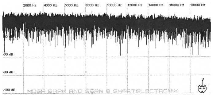

Figure 21. White noise routed through a low-pass filter. Higher frequencies have been attenuated while lower frequencies pass through.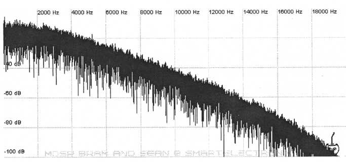

Another common filter type is the high-pass filter. This filter as the name implies works by attenuating low frequencies and passing the high ones. Some natural sounds have diminished or outright lack lower-pitched harmonics. Isn’t this impossible given that the pitch of a note is determined by the frequency of its lowest harmonic the fundamental? Remember that the frequencies of overtones are related to the frequency of the fundamental. If the fundamental and some of the lower overtones are missing our brains are able to relate the frequencies of the existing higher overtones back to the missing fundamental and perceive the correct pitch. This type of filter can be useful for recreating cymbals, handclaps and other instruments that sometimes lack lower frequencies.

Figure 22. White noise routed through a high-pass filter. Lower frequencies are attenuated while higher frequencies pass through.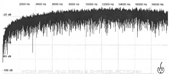

Two other filter types that are related to one another are the band-pass and band-reject filter. A bandpass filter attenuates both high and low frequencies and only lets a narrow band of frequencies through.

Figure 23. A band-pass filter only allows frequencies within a narrow band to pass.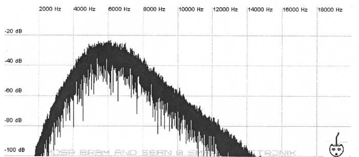

A band-reject filter, or notch filter, is essentially the inverse of the bandpass filter. It lets high and low frequencies pass and attenuates frequencies within a narrow band.

Figure 24. A band reject filter removes frequencies within a narrow band but allows all others to pass.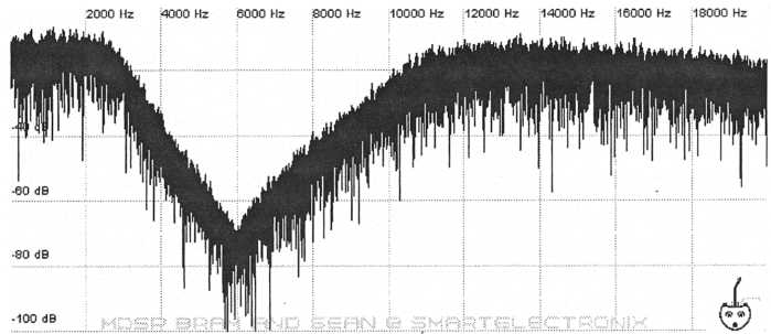

Cutoff Frequency

The cutoff frequency sets the frequency point where filtering begins to take place. If for example a low-pass filter has its cutoff frequency set to 6 khz then the output will pass all frequencies below 6 khz and all higher frequencies will be diminished. In actuality some filtering actually takes place at frequencies before the cutoff frequency. To be a bit more strict with our definition the cutoff frequency is usually taken to be the point at which the frequencies have been attenuated by -3 db, but this can be slightly different from one instrument to another.

Figure 25. Here cutoff frequency has been set to 6 kHz (6000 Hz). Notice that frequencies less than 6 kHz are also filtered but to a lesser extent than those above 6 kHz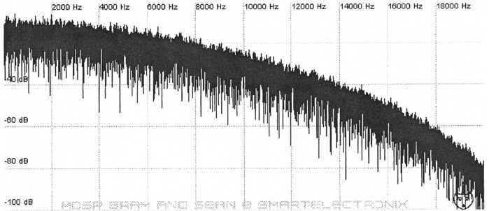

Filter Slope

A common misconception with filters is that all frequencies beyond the cutoff frequency are removed from the signal. The filtering beyond the cutoff frequency actually takes place gradually. The rate or degree of filtering that takes place beyond the cutoff frequency is determined by the slope of the filter. The most common types are 12 db

and 24 db per octave slopes and occasionally 6 db, 36 db and other values are used. A larger decibel value means more attenuation. A 12 db low-pass filter will sound slightly brighter than a 24 db low-pass when set to the same cutoff frequency. What these values mean is that for every octave the frequencies will be attenuated by the given decibel amount. For example let’s say we have a 24 db low-pass filter and the cutoff frequency is set to some fairly low value like 1.5 kHz. Let’s compare the filtering at 4 kHz and 8 kHz since these values are both in the filtered region. Frequencies at 8 kHz will be 24 db “quieter” than those at 4 kHz since these frequencies are one octave apart.

Figure 26. Filter response of a 24 dB per octave low-pass filter. Material at 8 kHz is attenuated 24 dB more than material at 4 kHz since these frequencies are one octave apart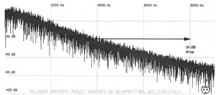

Filters are also referred to by their number of “poles.” One pole equals 6 dB of filtering. A two-pole filter is the same thing as a 12 db filter. A four-pole filter is the same thing as a 24 db filter.

Figure 27. Filter slope of a 2-pole, 12 dB per octave filter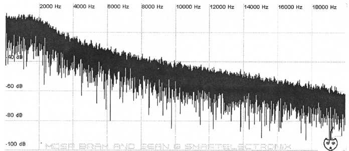

Figure 28. Filter slope of a 4-pole, 24 dB per octave filter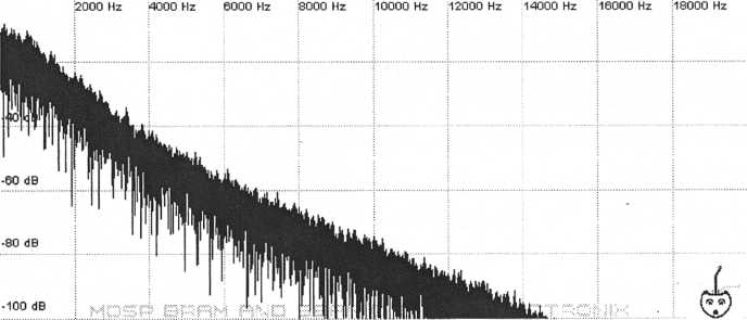

Some synthesizers allow the user to select various filter types. No type is inherently better than another and the most preferable type depends upon the application.

Resonance

Figure 29. Filter resonance at a 4 kHz cutoff frequency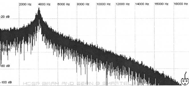

The function of the resonance setting on a filter depends upon the filter type. Its purpose is completely different in low and high pass filters than it is in band-pass and band-reject filters. When used with either a low-pass or a high-pass filter, resonance amplifies those frequencies closest to the cutoff frequency. When used with band-pass and band-reject filters the resonance setting acts as a “Q” control and sets the width of the band.

It should be made clear that resonance on a synthesizer is not the equivalent of resonance of an acoustic instrument nor is it necessarily used to replicate the resonance of an acoustic instrument. In situations where a particular frequency or set of nearby frequencies need to be amplified resonance becomes a useful tool.

Most synthesizers have gain compensation which will automatically lower the overall output of the signal as resonance is increased. This helps to prevent the resonant spike from going through the roof but it comes at the expense of lowering the rest of the signal.

Figure 30. Increasing the resonance results in gain compensation automatically lowering the amplitude of surrounding frequencies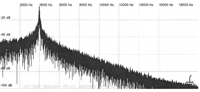

Some filters are self-resonating meaning that when the resonance is turned up high the filter will resonate even if no signal is input into the filter. This effectively turns the filter into a sine-wave oscillator. If keyboard tracking is available on the filter then this sine wave can be played as if it were a waveform from one of the oscillators. In cases where a synth does not have a self-resonating filter it is still possible to “play” the filter’s resonance with keyboard tracking by feeding a noise source into the filter and using this to drive the filter’s resonance.

Another way to play a resonant filter directly is through a method employed in acid electronica. The acid genre got its name not as a drug reference but rather from what are known as acid lines or acid tracks. Acid lines in turn got the name due to the way they sound. The acid line is one of those great stories in electronic music where a technology, in this case the resonant filter, is used in a fashion not originally intended. More specifically it was born out of the Roland TB-303 in the mid 80s. The “303” was originally marketed as a bass accompaniment for guitarists. It is essentially a sequencer that plays a single oscillator and was never intended to be played in a realtime or improvisational sense. The unexpected thing that happened was that electronic artists learned to use the TB-303 as a realtime instrument by turning up the resonance and alternating the filter cutoff frequency manually in realtime thus changing the pitch of the resonance while the unit’s onboard sequencer cycled thorough note patterns.

Here’s an example of how to create a very basic acid line without having to sell vital organs to buy a TB-303. Program a sequencer to loop through a rhythm that consists of only one note. Most acid tracks don’t use just one note but we’ll do it here just to better illustrate the process. The synth’s oscillators can be set to any waveform but I’d suggest using a sawtooth. Turn the resonance up to about 3/4 of its full position. Now as the sequencer plays, the synth alternate the filter cutoff frequency by hand. This will cause the pitch of the resonance to change. You may have to confine the extent over which you twiddle the cutoff frequency to the lower part of its range as higher frequencies may be inaudible. Twiddle the cutoff frequency knob in time to the rhythm and there you have an acid line albeit a simple one.

ENVELOPES

Envelopes are used to control how various parameters change over time once a key is played. Envelopes can be used to control just about any parameter, but the most obvious use of an envelope is to control the way a patch’s amplitude changes. If we want a patch to start loud and die out slowly like a cymbal or start out quiet and slowly become louder like a violin an envelope could be used to control the amplitude.

Figure 31. Representation of an ADSR envelope. ADSR envelopes can be applied to many different parameters but are most commonly used to control amplitude and filter cutoff frequency.

The following graph shows the effect that an ADSR envelope can have on amplitude.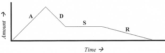

The most common type is the ADSR envelope which breaks the time over which a key is struck and held into four distinct periods called stages. ADSRs are hence known as four- stage envelopes. “A” stands for attack and it controls the rate of the envelope’s initial increase. “D” is for decay and it controls the rate at which the envelope decreases after the attack. “S” is for sustain and this controls the level at which the envelope will remain until the key is released. “R” is for release and it controls the amount of time that it takes for the envelope to die out after the key is released. Attack, decay, and release all control lengths of time and settings are commonly given in seconds and milliseconds. Sustain on the other hand sets the level after decay has completed and has no set time associated with it. It begins as the decay ends and will last indefinitely until the key is released. It’s sometimes given as a percentage where 100% would be the maximum setting.

Figure 32. The results of an ADSR envelope controlling amplitude as viewed in the sound editor Audacity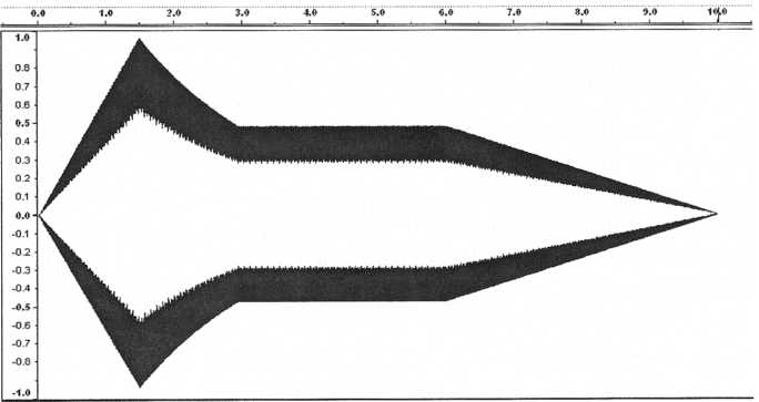

Incidentally, if sustain is set at 100% then decay really serves no purpose as it will not “decay” down. There are also variations on the ADSR configuration. The original MiniMoog used an ADS envelope where the “Decay” setting also doubled as a release setting. The ARP Odyssey and ARP 2600 had AR envelopes as well as the conventional ADSR type. There are also envelope types that use more than four stages but the ADSR is the most common.

Another use for envelopes is to control the filter’s cutoff frequency. If you listen closely to woodwinds or brass instruments you may notice that as the player begins to blow into the instrument that not only does the amplitude increase but the sound also becomes brighter. As pressure builds in the instrument higher frequencies are added to the sound. These higher frequencies are also the first to die out when the player stops blowing. This behavior can be replicated by controlling the filter’s cutoff frequency with an envelope.

Here’s a piece of advice to give a patch more character and realism. Use the filter’s envelope to create changes in the amplitude and then use the amplitude envelope to make any remaining adjustments. Huh? You may be asking why and how the filter envelope can be used to control amplitude. Isn’t that what the amplitude envelope is for? Well, it’s simple really. Whenever frequencies are removed from a signal they no longer contribute to the overall power of the signal. Removing frequencies will result in an overall lower amplitude. A filtered signal isn’t as loud as an unfiltered signal. Because of this a filter envelope has the effect of behaving somewhat like an amplitude envelope. This approach can be restated as the following. First use the filter envelope to control the amplitude of the higher harmonics and after that use the amplitude envelope to control the amplitude of the remaining lower harmonics that were untouched by the filter.

The filter envelope has an amount setting that is used to determine how much the envelope influences the cutoff frequency. Sometimes it can be a bit tricky deciding whether to adjust the cutoff frequency or the envelope amount. In these situations the best suggestion is to experiment by adjusting both.

To compare the amplitude and filter envelopes try the following. Set the oscillators to produce any waveform that you like. With the filter completely open (i.e. no filtering) raise the attack amount up on the amplitude envelope. You should hear the sound slowly get louder as you hold down a key. Now turn the amplitude attack back down and this time lower the filter cutoff frequency, increase the filter envelope amount, and increase the filter envelope attack time. As you hold down a key notice that the sound gets louder just as before but this time the timbre or tonal quality of the sound also changes.

LFOs

LFO stands for low-frequency oscillator. Unlike a synth’s main oscillators an LFO is not heard at the output or at least not directly. It is a modulation source meaning that it is used to create changes in other parameters. LFOs are used to create cyclic fluctuations in pitch, amplitude and a variety of other parameters. To add vibrato or tremolo to a patch an LFO would be used to modulate the pitch and amplitude respectively. Another key difference is that the main oscillators produce waveforms with frequencies in the audible range of 20 Hz - 20 kHz while LFO frequencies are typically less than 20 Hz. If an LFO could be connected directly to the output it would be inaudible because of its low frequency.

LFOs are similar to the main oscillators in that they do use square, triangle, and sawtooth waves and they also commonly use sine waves and sample & hold patterns. These are all referred to as source waveforms. Sine and triangle waves are the most ideal for imitating natural effects such as vibrato and tremolo. The results they produce, when used with an LFO at least, are very similar and for this reason it is not uncommon that a synth provides one and not the other.

LFOs have a frequency or rate setting that changes the speed of the cycle. Vibrato, tremolo typically use LFO frequencies under 5 Hz. Higher frequencies can be useful for many synthetic sounds and rhythm effects. The degree to which the LFO modulates a given parameter is controlled by an amount setting. Amount settings may either be found in the LFO section itself and sometimes they are located in each section to which they control.

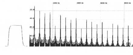
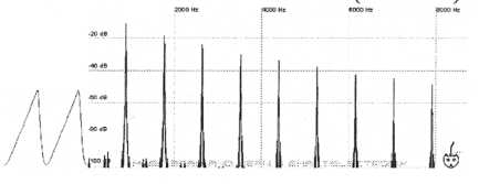
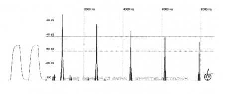
Following is the same patch played with the amplitude modulated by the LFO set to use a sine wave at 4.5 Hz. This creates vibrato.

Let’s look at what happens when an LFO uses a sine wave to modulate the amplitude of a patch. Here is a waveform of a patch without any LFO modulation.

Figure 33. A patch without any LFO modulation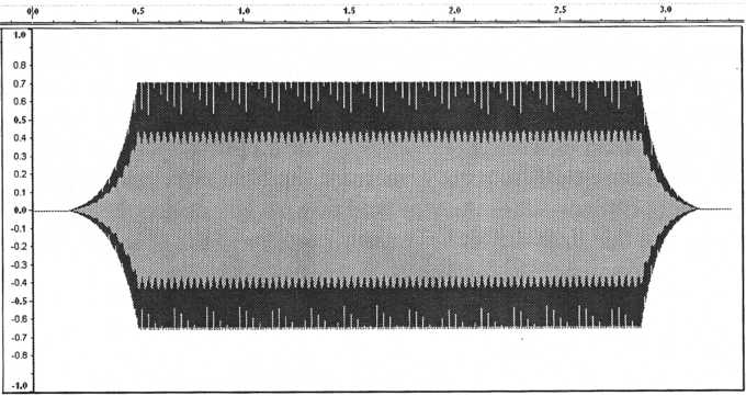

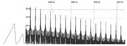
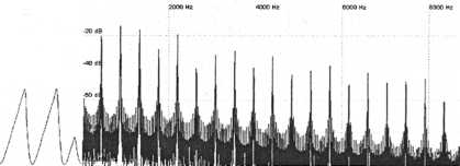
Figure 35. Patch with LFO modulation using a triangle wave source set to a frequency of 4.5 Hz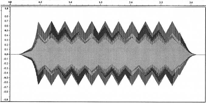

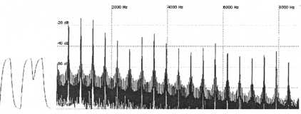
Figure 34. Patch with LFO modulation using a sine wave source set to a frequency of 4.5 Hz

In the next graph the LFO has the same frequency but uses a triangle wave.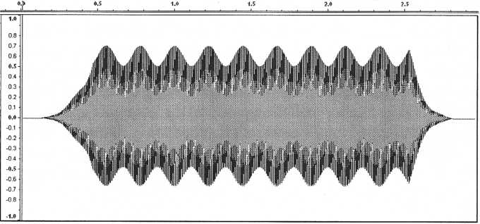

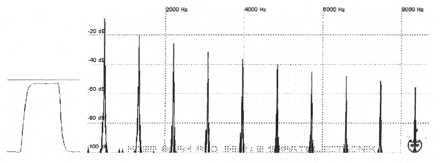
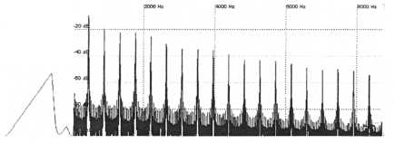
The sine wave source and the triangle source produce very dissimilar graphs but if you set your synth up to modulate amplitude and compare the use of a sine versus a triangle you will hear very little difference. When setting up the frequency of an LFO remember that 1 Hz = 1 cycle per second. In the above example the frequency was set to 4.5 Hz thus producing 4.5 cycles each second as can be seen by looking at the graphs.

Pulse-width modulation

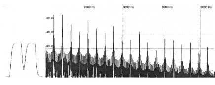
One of the coolest uses of the LFO is to create pulse-width modulation. Recall that changing the width of a pulse changes its harmonic content. Routing an LFO, using a sine or triangle source, to modulate the pulse width creates an extremely rich sound that could best be described as a thick, string section-like sound.

Below is a graph showing the harmonics of a pulse-width modulated waveform. Notice that the higher harmonics are broadened. This is very similar to the effect heard by chorusing or unison. Keep in mind though that pulse-width modulation tends to even out the levels of the harmonics. For instance a pulse that is set to a width of 25% will have harmonics that appear to undulate in amplitude. If a heavy dose of modulation is applied to the pulse width this undulation will disappear and the harmonic amplitudes will take on characteristics similar to that of a sawtooth that has some chorusing or unison.

Figure 36. Pulse-width modulation causes the upper harmonics to broaden resulting is a chorusing effect. This is very useful for string and pad sounds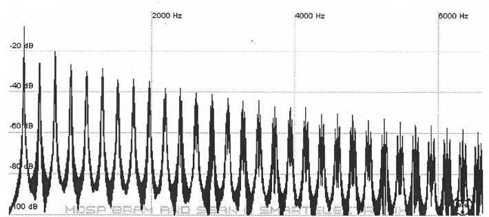

The trick to getting good PWM string sounds is to use pulse-width modulation on both oscillators and detune one about 10 cents high and the other about 10 cents low. Set the LFO frequency a bit under 5 Hz and the amount to a bit under 50% which will make it thick while minimizing the beating effect that is characteristic of PWM. Then apply some light chorus and delay if available.

Beat effects (gating and note switching)

Because of their cyclic nature, LFOs can also be used to create rhythm. This is where the square and sawtooth sources become the most useful. Using either one of these sources and routing the LFO to modulate the amplitude or filter cutoff frequency can result in useful gating effects. Using a square wave source will cause the output to have a repeating On/Off pulsing pattern. A sawtooth source will cause the sound to cycle through a “ramp up” or “ramp down” depending on the direction of the sawtooth. These effects are particularly useful when the LFO frequency is matched to the beat of the song. A common attribute of LFOs on many modem synthesizers is the ability to sync to a time signature provided either internally or by an external sequencer.

By routing a square wave source LFO to modulate pitch it is possible to create note switching, trill sounds. The key here is to set the LFO depth to something that will produce a musically useful interval such as a fifth (7 semitone difference) or an octave (12 semitone difference). This can be a useful way to create a simple two-note arpeggio/trill effect that can be useful particularly if your synth lacks an arpeggiator.

KEYBOARD EXPRESSION

Sample & hold

Without getting into a deep explanation sample & hold is a random pattern that is often available as an LFO source. It’s great for creating the computer-type sounds from old sci-fi movies. Set the LFO source up to be sample & hold (or noise) and route it to modulate the oscillator pitch. This should produce a cheesy computer sound. Also try routing the LFO to the filter cutoff frequency and turn the filter resonance up. This produces a different but equally as cheesy computer sound!

Sync sweeping

Here’s a great way to use an LFO to create a screaming, growling lead. Set the slave oscillator to sync to the master oscillator. Keep the master oscillator turned on but keep its volume all the way down. Tune the slave oscillator higher than the master’s pitch.

Set the LFO to use a sine or triangle at a really, really low frequency (<1 Hz) and use this to modulate the slave’s pitch. Apply portamento (glide) and lay on some unison and chorusing. Experiment with different LFO frequencies and depths. As you increase the LFO amount decrease the LFO frequency.

Keyboard Expression

Velocity Sensitivity

If a piano’s keys are struck hard it will obviously sound much louder than if they are struck lightly. Not only that but the timbre of the sound will be much different as well.

A hard-struck piano doesn’t simply sound like a louder version of a lightly-struck piano. Both the amplitude and harmonic character of the sound depend on how hard the keys are played. This type of behavior can be replicated on synthesizers that have velocity sensitive keyboards. A velocity sensitive keyboard can be used to modify parameter amounts based on how fast the keys are pressed. The two most common uses for velocity sensitivity are to change the amplitude level and the filter-cutoff frequency, but it is also sometimes used to modify pitch, envelope times, LFO rates and amounts, and just about anything else. Velocity sensitive keyboards allow for much greater expression and realism. These days most keyboards have velocity sensitivity but not all do particularly inexpensive ones and even pro models produced before the mid 80s. Be sure to check before buying that next synth.

Aftertouch (pressure sensitivity)

A keyboard with aftertouch or pressure sensitivity allows the user to control parameter amounts based on how much pressure is applied to the keys as they are being held down. This can be quite useful when used with the filter to imitate wind instruments being overblown or routed to pitch for replicating string bending on a violin. Like velocity sensitivity it to can be applied to a wide range of parameters. Aftertouch keyboards come

KEYBOARD EXPRESSION

in two different flavors. The cheapest to implement and therefore the most common is channel or global aftertouch. A keyboard with channel aftertouch averages the pressure from all the depressed keys to create a single aftertouch message. Polyphonic aftertouch which is much more rare allows each key to transmit its own aftertouch message. While it has become more common, most keyboards do not have aftertouch so if this is something that interests you be sure to look for it.

SYNTHESIS THROUGH HARMONIC ANALYSIS

Synthesis Through Harmonic Analysis and Reverse Engineering

The use of harmonic analysis in synthesis is nothing new, yet it has not been used much outside of academic research and professional patch programming. There are a few reasons for this. The first is that harmonic analysis requires a fair amount of processing power that until recently was too expensive for most of us. Fortunately home computers are now powerful enough to perform the analysis in real-time while using only a small percentage of the computer’s processor. The second reason is that it is generally perceived as difficult to use. There is quite a bit of mathematical theory that goes into computing the Fast-Fourier Transforms (FFT) on which harmonic analysis is based but as far as using harmonic analysis as a tool for synthesis it’s rather straightforward. The third reason, somewhat as a result of the first two, is that it simply hasn’t become part of convention.

This is super powerful stuff and it has the potential to change the way you program sound. Even though this section is centered on analyzing harmonics and reverse engineering musical content it should be noted that it will also improve your ability to create original patches as well. After you use it for a while and you come to understand the spectral makeup of different sounds you will rely less and less on having to look at harmonic diagrams. They’ll be in your head. This book is about analog synth programming but it should be mentioned that harmonic analysis also makes FM synth programming infinitely easier to understand. Don’t even bother programming FM without it! I digress...

Before proceeding I recommend that you first get a hold of software that can perform harmonic analysis/FFT in realtime and play around with it for a bit. Most of the more sophisticated sound editors provide the ability to display harmonic diagrams of sound files albeit usually not in real-time. For real-time analysis I highly recommend the Fre(a)koscope VST plug-in. This plugin was used to create all of the harmonic diagrams in this book. It has an excellent interface, is easy to use, and it’s free! If you don’t have a host that supports VST plugins be sure to visit kvraudio.com where you can find a number of hosts available for free. If you have any questions please email me at synthcookbook@yahoo.com

The analysis/synthesis process can be broken down into three stages for each sound.

1. The most important step. Obtain a harmonic diagram of the sound that is to be emulated or recreated. Pick the best oscillator waveforms, pitches, and amplitudes to match the diagram.

2. High frequency harmonics are generally the last to rise in amplitude and are the first to die back out. While comparing with the harmonic diagram of the original source use the synth’s filter envelope to match this behavior.

3. Using a sound editor, match the synth’s envelopes to the original source.

Step one is essential while steps 2 and 3 are not always possible or required. Envelopes may not require any visual analysis since they can be duplicated by ear with good results more easily than harmonics. Note: The lowest-pitched harmonics are the most important. As a general rule of thumb try to get the first 5-10 harmonics as close to their corresponding levels in the original source.

Reverse engineering a patch from another synth:

The easiest sounds to recreate are those from other analog synths. Because analogs have very similar feature sets it makes for easier translation. About ten years ago I had to sell a Sequential Circuits Six-Trak but I made sure to record samples of some of my favorite patches that I’d programmed for it. My favorite was a lead with thick unison and we’ll begin by reverse engineering this patch. The sample of this patch can be found on the CD.

Playing the sample through Fre(a)koscope produces the following harmonic diagram,

Figure 37. Harmonics of a patch originally programmed on a Sequential Circuits Six-Trak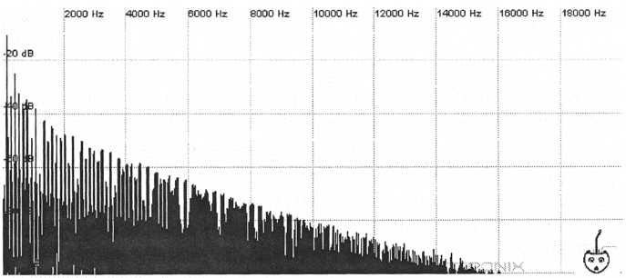

Here Fre(a)koscope has been set to a linear display and a maximum window size with a frequency range of 20 Hz - 20 kHz. The lower harmonics are the most important so let’s decrease the maximum frequency of the display so that we can see these in greater detail. Lower the maximum range down to about 6 kHz.

Figure 38. Six-Trak patch zoomed in to show finer detail in the lower-frequency harmonics. The pitch of the sampled note is at C3 on the keyboard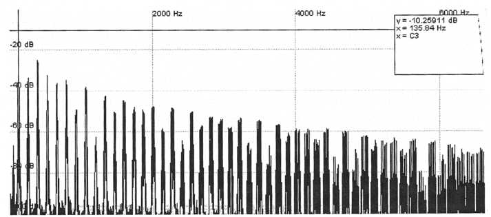

In Fre(a)koscope it is possible to get decibel value, frequency, and equivalent key number by clicking on a section of the graph. In the graph above the fundamental has been selected and from the inset box at the upper right we see that the sample is tuned to the C3 key. We need to know this so that we know what key to play on the synth that is

being programmed. There are many important details in the above graph that give us a clue as to where we should start. Notice that both even and odd harmonics are present. This rules out using a single triangle wave or square wave since they have only odd harmonics.

The two remaining options are sawtooths and pulses since they possess both even and odd harmonics. Also notice that the higher harmonics become broad and are not the narrow spikes that we would expect with pure sawtooths or pulses. This indicates that there could be some pulse-width modulation taking place or the oscillators have been set to unison. We will get back to the broad harmonics in a bit but for now look at the way the harmonic amplitudes do not decrease evenly from left to right. A sawtooth that has been synced can produce harmonics that look like this but so can a pulse with variable width. Let’s take a look at the synced sawtooth option first. Set your synth up with the slave oscillator synced to the master oscillator and have the slave produce a sawtooth wave while at the same time the master’s output is turned all the way down. Increase the pitch of the slave while keeping an eye on the synth’s harmonic analysis. The closest that we can get to the original harmonics this way is when the slave oscillator is tuned about 8 semitones above the master.

Figure 39. A synced sawtooth oscillator tuned 8 semitones above the master produces results similar to the original patch but not close enough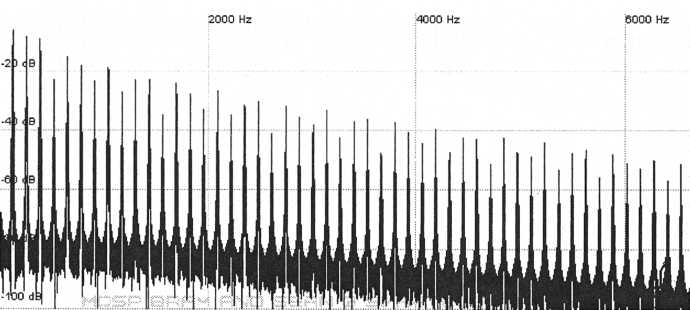

What are the notable differences between this graph and that of the original Six-Trak sample? Of course the harmonics are all narrow and again we will get to that in a moment but for now we only need to compare their amplitudes to the original patch. The higher harmonics in our patch are slightly louder than those in the original. Notice that they are higher on the graph. This can be remedied by applying some low-pass filtering but there is a bigger discrepancy than this. Notice that the harmonics of our patch do not undulate up and down in quite the same fashion as the original patch. It would however be a good guess that if we find out what is broadening the higher harmonics of the original patch and we apply it to our patch as it is right now that the two would nonetheless sound very similar but we are going to try to do better. Remember this was originally produced by another synthesizer so we should be able to get really close and we can probably even nail it.

Let’s see what we can come up with using a pulse instead of a sawtooth. Again only use one oscillator but this time do not sync it to the other. Set it up to produce a pulse. Begin by setting the pulse width to produce a square wave. Remember that a square wave should only show odd harmonics. Now very slowly begin decreasing the pulse width. Before the width has been decreased much at all you should get harmonics that are identical in amplitude to those of the original patch. This happens to be at a pulse width of about 44%, something not much narrower than a square wave but harmonically different. Now we haven’t yet applied any filtering so the harmonics will not diminish quite as rapidly as those in the original patch but the levels of each harmonic relative to their neighbors follows the same pattern as those in the original.

Figure 40. A pulse width of 44% produces harmonics that are very similar to the original patch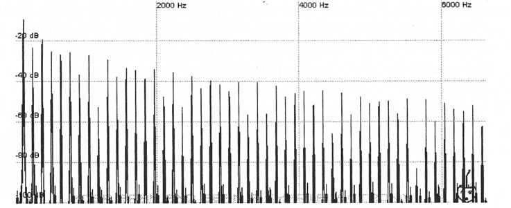

Next experiment with some low-pass filtering until the level of the higher harmonics matches those of the original. A 24 dB filter set to a cutoff frequency of 2.5 kHz produces the following graph.

Figure 41. Apply some low-pass filtering to match the harmonic amplitudes to those in the Six-Trak patch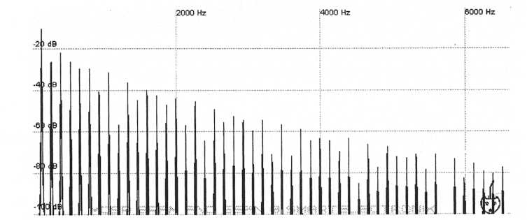

There are some differences between this and the original but the amplitudes are pretty darn close. While two synths can produce practically the same results they cannot produce exactly the same results.

The one last thing that we need to take care of is determining what is causing the higher harmonics to broaden. This could either be due to pulse-width modulation or oscillator

unison. Try applying some pulse-width modulation. As the pulse-width modulation amount is increased it produces the following results.

Figure 42. Pulse-width modulation broadens the higher harmonics but it also flattens out the harmonic amplitudes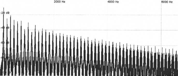

This has broadened the higher harmonics as we had hoped but it has also managed to decrease the amount of undulation in the harmonics. Pulse-width modulation obviously wasn’t used in the original patch.

Figure 43. The harmonics of the resynthesized patch in its final form

This is very similar to the original

Figure 44. The harmonics of the original patch

Get rid of the pulse-width modulation and this time turn on unison. The Six-Trak had six oscillators so set your unison mode to six oscillators if applicable. If you’re using the SCB synth turn unison mix and intensity all the way up and put speed at about 50%. You should get harmonics similar to those below.

Listen to the resynthesized patch and compare it to the original sample. They are practically indistinguishable. This also sounds far better than trying to stretch a 4 second sample across the whole keyboard using a sampler! If we wanted to do something like decrease the amount of filtering we can do that with the resynthesized patch but would not be able to using the audio sample.

Reverse engineering a sound from a song:

The tricky part to reverse engineering a sound that’s in a song is the presence of other interfering material. Here the goal is to find a clip of the sound that is as isolated as possible from other competing sounds in the mix.

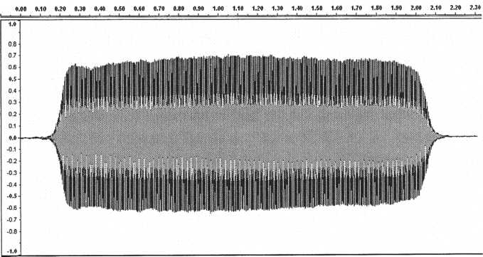
For an example of reverse engineering a sound from a song we’ll lift one off of Shape 1 from the Shape album which can be found on the CD. There’s a cool bass that starts at about 2:45 into the song. Use a waveform editor to take a look at the region from 2:45 to 2:50. An audio clip of this section can also be found on the CD. For waveform editing, I use Audacity which is an excellent freeware sound editor.

Figure 45. Audio clip containing the bass sound that is to be duplicated as well as a bass drum and even the tail end of a pad. The bass sound must be isolated from a section of this recording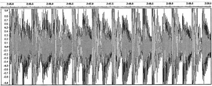

In this section there are three different sounds. There is the bass sound that we would like to isolate for resynthesis, a bass drum, and at the beginning of the section there is the tail end of the pad-type sound from earlier in the song. The bass and the bass drum both play ten times in the clip shown above. The bass is the quieter of the two. Because of the interference of the pad at the beginning of the clip we will isolate one of the bass voicings found after 2:47. Let’s take the one from region 2:47.79 to 2:48.04 . Yes that’s right, we are going to recreate the patch from a mere 1/4 second of sound!

Figure 46. Audio clip of the bass sound isolated from the region 2:47.79 - 2:48:04

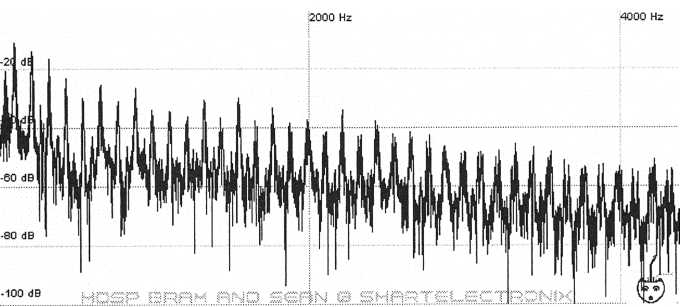
Figure 47. Harmonics of the isolated bass sound. The high noise floor is the left overs of other sounds and effects in the mix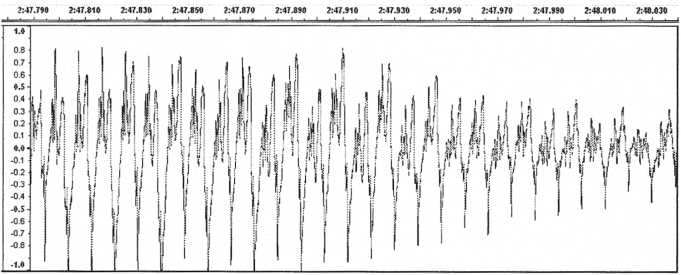

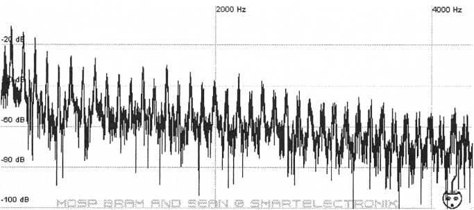
Running this clip through a harmonic analyzer set to a linear view produces the following harmonic diagram. The range has been set to show the lowest harmonics.

Notice that the noise floor isn’t very far below the tops of the harmonics. This is most likely the left over garbage from other sounds and effects in the mix. Look at the far left of the diagram and at what appears to be the first harmonic. The dark nub just below the -20 dB line. This too is most likely an artifact since its frequency doesn’t relate to any of the other harmonics. If this were a sample of an acoustic instrument this statement might not be true but the one thing we know about this sample is that it came from another synthesizer which most likely used standard waveforms having harmonics at evenly- spaced frequency intervals.

As in the previous example we need to determine the pitch of the sample so that we know what key to play on the keyboard. In the case of Fre(a)koscope the cursor indicates that it is pitched to the A2 key. There are some similarities between this diagram and the one of the original Six-Trak patch back in the preceeding example. Like before, the broadening of the harmonics at high frequency indicates the presence of oscillator unison so we will want to turn that on. Here we also have undulating harmonics but unlike the previous example there is more of a pattern to the way they go up and down in amplitude. Notice that from about 1000 Hz to just above 2000 Hz that every other harmonic is lower than its neighbor. Also in the earlier example some harmonics were drastically diminished while others were only slightly. Here the change in amplitude is more uniform. These are

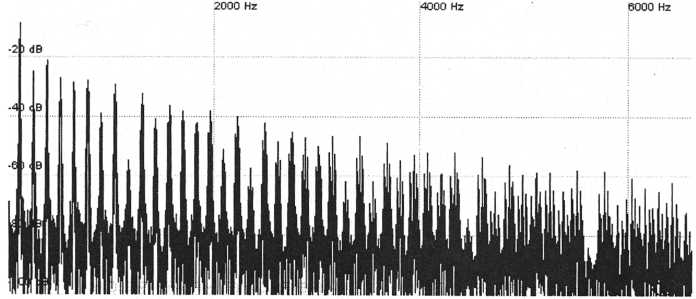
tell-tale signs that we are looking at a sawtooth wave mixed with either a second sawtooth or a square wave and not oscillator syncing or pulse-width modulation. The reason that one of these must be a sawtooth is that if we use just square waves or triangle waves, which have only odd harmonics, no matter how they are detuned from one another there will always be some missing harmonics. In the graph above there are no missing harmonics. Try playing with just square and triangle waves and detuning one of the oscillators to move its harmonics around. You’ll find that no matter how the tuning is changed there are always missing harmonics.

We must now determine what waveform is used by the second oscillator as well as its pitch. Look at the harmonics of a single sawtooth tuned to A2 with unison and compare it to the harmonics of the sample.

Figure 48. Sawtooth wave tuned to A2 with unison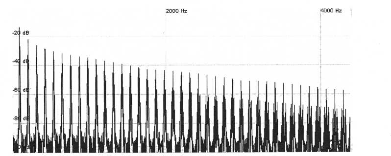

We need to increase the amplitude of the even harmonics while leaving the odd harmonics unchanged. A square wave won’t work because it is made of only odd harmonics. If we add a square wave to the sawtooth we get undulating harmonics but they are in the wrong order and the sound doesn’t have the same bite as the original. Here is a graph of that.

Figure 49. A square wave added with a sawtooth produces undulating harmonics but they are in the wrong order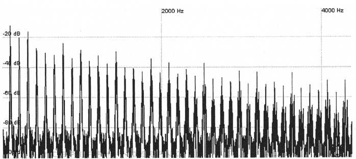

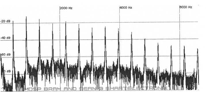
If we tune the square up an octave its even worse. Now every fourth harmonic is increased starting at harmonic two.

Figure 50. If the square wave is tuned up an octave the results match even less than before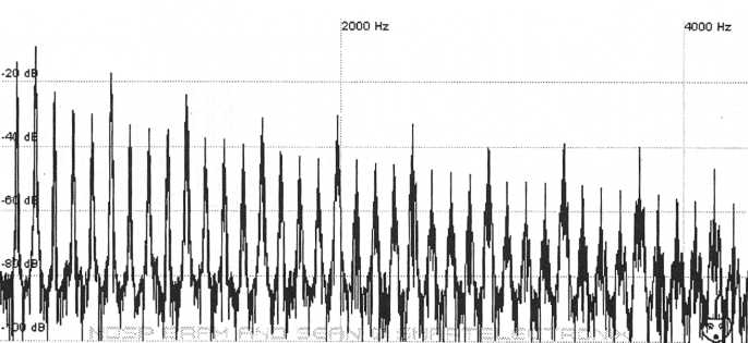

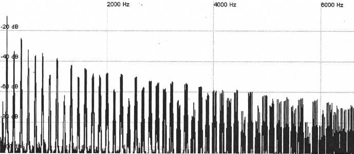
The square wave doesn’t work so we’ll have to try using a second sawtooth. This second sawtooth must be tuned up one octave. Why? Everytime a sound is tuned up an octave not only does the frequency of the fundamental double but more importantly for this particular situation the frequency distance of the overtone harmonics also doubles. Here are the harmonics of a sawtooth pitched to A3

Figure 51. Harmonics of a sawtooth tuned up an octave to A3. Notice that the distance between harmonics has doubled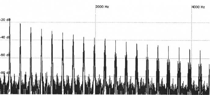

Notice that the harmonics are twice as far apart as those in the A2 sawtooth diagram. If we add the A2 sawtooth and the A3 sawtooth we will get the correct undulating harmonics.

Figure 52. Two sawtooth waves tuned an octave apart are used to create the final product

Figure 53. Harmonics of the original sample.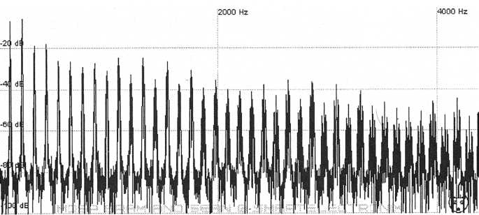

Compare this to the original.

The majority of the harmonics are within 5 dB of the positions in the original and the undulating pattern is the same. There are slight differences but again these are to be expected since no two synthesizers are exactly the same. Set the attack and release times of the amplitude envelope to zero for a good bass patch. Compare the sound of the original to our new patch and notice they are very similar.

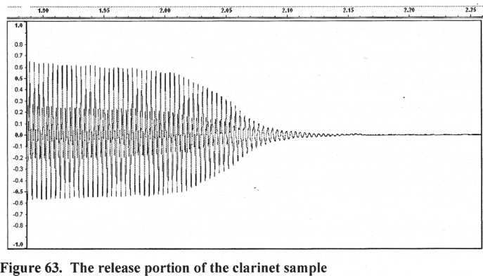
Emulating an acoustic instrument’s harmonics and envelope: Clarinet

In this example we will not only imitate the harmonics of the instrument but we will also use the filter envelope to recreate the original envelope. Here we will recreate the sound of the clarinet taken from a sample provided by the royalty-free online sample library of the University of Iowa Electronic Music Studios

(http://theremin.music.uiowa.edu/MIS.html). This sample can also be found on the CD.

Recreating the harmonics of acoustic instruments is more subjective than recreating patches produced by other analog synths. When recreating a synth patch we are basically trying to determine the settings of the synth from which it originally came and the end result is usually quite similar to the original. In the case of acoustic instruments however there are usually multiple ways to achieve harmonics that are similar to the original but with slight differences between the various methods. One method may do an excellent job of recreating the very lowest harmonics while another does a good job with higher harmonics. Recreating this clarinet as you will see is no exception.

Acoustic harmonic spectra are usually more complicated than those of analog synths.

The goal is to match the synth’s output as close as possible to the acoustic instrument while expecting to make sacrifices in one area of the audio spectrum to improve quality in other areas. The harmonics with the lowest frequencies are the most important. Take a look at the spectra of the clarinet.

Figure 54. Harmonics of a clarinet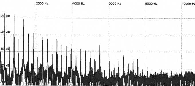

Here are the major details of the graph: The fundamental has a frequency corresponding to C4, harmonics 1,3, and 5 are dramatically louder than the rest, and there are not really any harmonics after 8 kHz. Even though there are both even and odd harmonics such as would be provided by a sawtooth, the first three odd harmonics (1, 3, and 5) stand above the rest. This sound can probably be duplicated by mixing a sawtooth with either a square or triangle since either of these have odd harmonics. Because none of the odd harmonics above harmonic 5 really seem to stand out would suggest that we try a triangle over a square since the triangle’s harmonics are quieter at higher frequencies. Here’s what you’ll get if you mix a triangle wave at full amplitude with a sawtooth wave -25 dB quieter than the triangle. Both at the same pitch.

Figure 55. A triangle wave mixed with a quieter sawtooth wave produces harmonics that are similar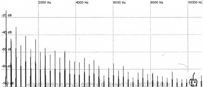

It sounds close and the harmonics look somewhat similar. There are probably clarinets out there that are nearly identical to this, but if we want to match this particular clarinet I think we can do better.

The way the first six harmonics undulate could be duplicated with a single pulse so let’s give that a try. Starting with a pulse width of 50% (square wave) and barely decreasing the width much at all (only down to 49%) we get the following harmonic diagram.

Figure 56. Pulse width set to 49%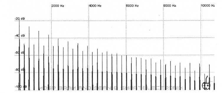

There is in fact hardly any difference between this and a square wave. A pulse width of 49% versus a width of 50% may have dissimilar looking harmonic signatures yet they sound practically identical. Sound wise this is really close and we’re probably splitting hairs to get closer but it is possible. We’ll use the pulse width to help produce the first three loud odd harmonics but now we have to figure out how to produce the rest. If we ignore the first three odd harmonics then harmonics 6 and 7 would be the loudest and all harmonics to the left and to the right of these would fall away getting quieter in both directions. How do we imitate this odd and peculiar behavior? Often the best way to make harmonics do odd and peculiar things in a patch is to use a synced oscillator. Here’s what we will do. Turn oscillator sync on and set the slave oscillator to use a square wave. Make sure the master oscillator is on but that its volume is turned all the way down at least to start with. We don’t want to hear the master but we do want the slave to be able to sync to it. Now, while looking at the harmonic output of the slave’s

square wave begin increasing the slave oscillator’s pitch up quite high and as you do you should notice that successively higher pitched harmonics become the loudest on the display. Keep increasing the slave’s pitch setting until it is 2 octaves and 5 semitones above the master and you should get harmonics similar to the following graph.

Figure 57. Output from a synced sawtooth tuned 2 octaves and 5 semitones above the master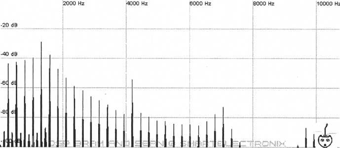

With the exception of harmonics 1, 3, and 5 this matches the original spectra closely. Now to finish out the sound set the master oscillator to produce a pulse with a width of 49% just like we did a few paragraphs back. Turn the volume of the master all the way up and turn the slave down to where it is rather quiet around -30 dB below the master and what you get should be similar to the following graph.

Figure 58. The master oscillator mixed with the slave oscillator

This is very close to what we want but the higher harmonics are still a bit loud so apply some low-pass filtering. A 24 dB filter set to a cutoff frequency of 2.5 kHz was used to produce the following result.

Figure 60. Harmonics of the clarinet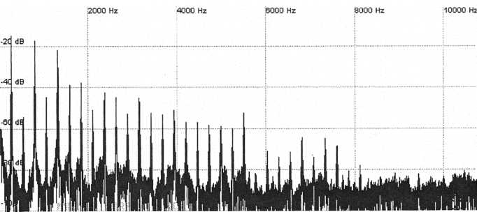

Figure 59. Applying some low-pass filtering to the mixed waveforms creates results that are very similar to the acoustic clarinet

Compare this to the original clarinet.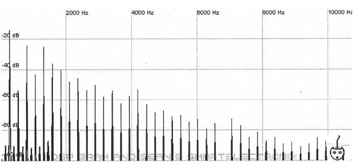

Since the first 5-10 harmonics are the most important we can consider our synthetic clarinet to be very similar to the acoustic clarinet. Not bad for old-school analog/subtractive synthesis! Call it good on the harmonics. Now lets move on to the envelopes.

Figure 61. Envelope of the clarinet

Here is the amplitude envelope of the clarinet in the audio sample.

We are going to duplicate this using the synthesizer’s filter envelope. Usually when a synth programmer looks at a waveform like the one above the first inclination is to duplicate it using the synth’s amplitude envelope. The above waveform is no doubt the natural amplitude envelope of the clarinet, however a more accurate reproduction of this envelope will actually use the synth’s filter envelope. Keep in mind that whereas the amplitude envelope changes the amplitude of all harmonics equally the filter envelope changes the amplitude of select harmonics. In the case of a low-pass filter, the filter envelope changes the amplitude of the higher frequencies more dramatically. Therefore, the filter envelope is after a fashion a form of amplitude envelope.

Listen to the very beginning of the clarinet sample on the CD where the player just begins to blow into the instrument. The most obvious thing that you’ll notice is that the amplitude of the note increases. Listen a bit more closely and you should also be able to notice that within that first fraction of a second the instrument sound becomes not only louder but also brighter. As the player begins to breath low-pitched harmonics amplify first followed by successively higher-pitched harmonics. As more and more high harmonics are added the overall sound becomes brighter and louder. At the end of the sample when the player stops blowing, the high harmonics are also the first to die out. This is true to varying extents in just about all instruments. Woodwinds in particular have a very strong relation between overall amplitude and amplitude changes of individual high harmonics.

Zooming into the beginning of the sample we see that the clarinet has an attack of about 0.15 seconds in length.

Figure 62. The attack portion of the clarinet sample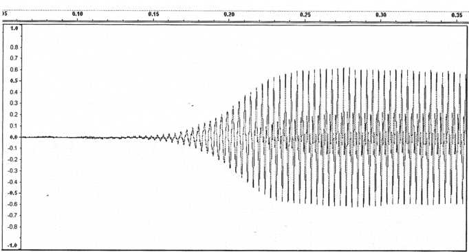

Zooming into the end we see that the “release” portion takes roughly 0.2 seconds

In the synthesizer set the filter’s cutoff frequency to its lowest setting, turn the filter envelope amount up to its maximum setting. Set the filter envelope’s attack to 0.15 s, release to 0.2 s, and sustain all the way up to 100%. The decay time doesn’t matter since sustain is at 100%. To keep the amplitude envelope from interfering make sure its attack is set to 0, sustain 100%, and release set to maximum. Now play a note on the keyboard. There’s now a gradual attack and release but the sound is way too bright. While holding down a key, reduce the filter envelope’s amount setting until the output sounds more like it did before we started messing with the envelope. To be a real stickler for accuracy look at your harmonic display while reducing the envelope amount until the higher- frequency harmonics are back where they were originally. Try playing it now and it should sound quite good.

Let’s now add a faint hint of vibrato. Look closely at the original waveform in Figure 61 and notice how there are shallow peaks and valleys. They are hardly pronounced enough to be considered true vibrato. Excuse the jargon but they’re more like quasi-periodic fluctuations caused by variations in the player’s breath with a period of about 0.05 seconds. Remember frequency is equal to one over the period so: 1/0.05 s = 20 Hz. So set the LFO to around 20 Hz and route it to the amplitude. Set the LFOs modulation amount to where it inst barely creates a vibrato effect. Around 2% is good if not less.

Figure 64. LFO used to create vibrato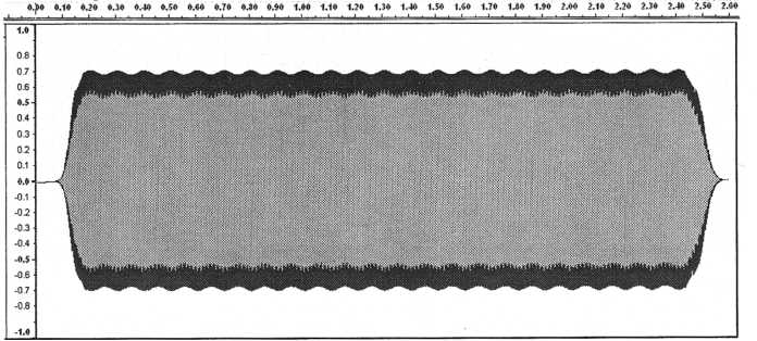

The attack and release are very similar and we were able to use the LFO to somewhat duplicate the amplitude fluctuations. It sound’s quite similar and we probably aren’t going to get much closer than this. This not only sounds like a clarinet, but it sounds like the specific clarinet from the audio sample. Harmonic analysis allows us to get exceedingly close to the original source material. Analyze the harmonics of your own voice and synthesize it. Trust me, it’s kind of creepy!

Compare this with the original.

Figure 65. Notice how closely the attack and release in fig. 64 match with the original. The LFO was used to mimic the slight amplitude fluctuation in the original clarinet sample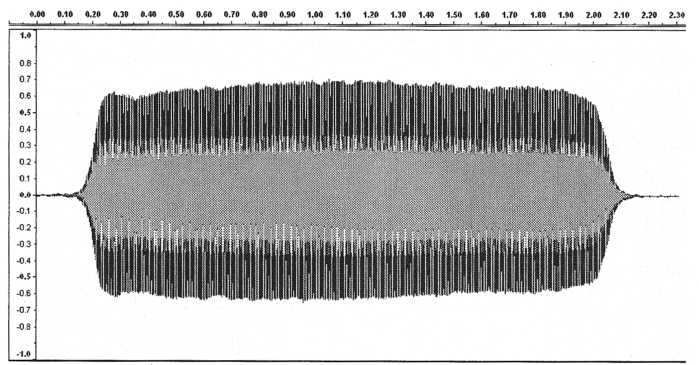

Ok, so the amplitude envelope wasn’t used. Why are synthesizers built with amplitude envelopes then? Like I said before, woodwinds like the clarinet have envelopes that are very dependent upon the amplitude changes of their higher harmonics. When synthesizing most acoustic instruments both envelopes are usually used. Most instruments do not have such an extreme change in timbre at the attack and release as woodwinds like the clarinet and therefore the amplitude envelope can be given more control on these patches. An amplitude envelope can also be used to change the contour of the overall envelope. Look at the attack of our clarinet patch for example.

Figure 66. Attack portion of the clarinet patch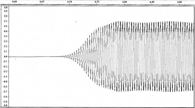

If we instead set both the filter and amplitude attacks to 0.15 seconds the overall attack will take the same amount of time but will come up more abruptly at the end of the attack.

Figure 67. Setting both the filter and amplitude attack times to 0.15 seconds changes the contour of the attack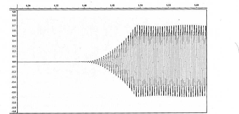

The filter attack and amplitude attack have been used together to change the contour of the overall attack. Though we don’t need to use this approach on the clarinet, it can be very useful for contouring the releases of percussion and plucked and hammered strings.

HOW TO PROGRAM THE COOKBOOK PATCHES

Oscillators

Wave : Waveform choices include sawtooth, square, triangle, and pulse width (PW). Pulse width values are given as a percentage of the waveform period. For instance a pulse width of 50% is a square wave and a pulse width of 25% is a pulse with a width that is half that of a square and sounds more “brassy.” Pulse widths greater than 50% are not included as they are just inverted versions of those between 0% and 50% and therefore sound the same. You will need to know if your synth’s pulse-width setting goes from 0%-50% or, more commonly, 0%- 100%. If you have a synthesizer such as the ImpOscar which uses values of 50%- 100% simply subtract the pulse width values in the book from 100 to get the value you need to use. If the synthesizer lacks the ability to set the pulse width of the square wave then substitute pulse-width values 0%-30% with a sawtooth wave and values from 30% - 50% with a square wave. If the synthesizer lacks a triangle wave then use a square wave in it’s place when called for along with slightly more low-pass filtering. Triangle and square waves sound similar because they are both composed of odd harmonics but the higher harmonics of the triangle are less audible.

Tune: Values are listed in octaves, semitones, and cents. This is the value by which one oscillator should be detuned from the other oscillator. For patches where both oscillators have a tuning value listed it is the amount by which each oscillator is to be detuned from a common pitch. If the tracking for oscillator 2 is turned off this field will list the specific pitch for which oscillator 2 is to be tuned.

Mix: This is the amplitude of the oscillator. Values are given in decibels where the maximum amplitude is 0 dB and quieter amplitudes are given as negative values. Some synthesizers display amplitudes where the maximum amplitude is not 0 dB. It may for instance be some positive value. In these cases just subtract the value listed in this book from the maximum value displayed by the synthesizer. For example if the synthesizer displays a maximum value of 13 dB

for the volume of one of the oscillators and the setting called for in this book is - 7 dB then the oscillator should be set to a value of 6 dB. It’s not that big of a deal just as long as you make sure the oscillators are separated by the same amount. The percentage to the right of the decibel value is the percentage of the maximum setting of the oscillator amplitude. This can be used for synthesizers that do not display values in decibels. Since oscillators on different synths have amplitude adjusters with different responses this percentage is a ballpark approximation and may require some adjustment by ear. For more accuracy it is best to calibrate the synths mix settings as explained in the last section of this book.

Oscillator 2 tracking: This is either on or off. When on the pitch of oscillator 2 will track the keyboard. When off oscillator 2 will play the same pitch on all keys.

Oscillator 2 sync: When on it syncs oscillator 2 to oscillator 1. You may need to check your synthesizer’s documentation to be sure which of its oscillators syncs to the other when syncing is turned on.

Noise

Noise: White noise source set to either on or off.

Mix: Amplitude of the noise source given in decibels. The statements made above in the section on oscillator mix apply here as well.

LFO

Routing: Sets the destination of the LFO. Destinations include amplitude, pitch, filter cutoff, and pulse width.

Wave: Waveform used by the LFO as a modulation source. Waves used are sine, triangle, and square.

Frequency: Sets the rate of the LFO. Values are given in Hertz (Hz).

Qualitative suggestions are given in italics.

Depth: Sets the amount by which the destination is modulated by the LFO. This is given as a percent of the settings range when modulating amplitude, filter cutoff, and pulse width. The knob/slider that controls depth would be turned half way for a depth of 50%. When pitch is set as the destination the depth is given in terms of the amount of pitch that a played note will vary.

Glide: Also known as portamento. Set to either on or off

Time: Glide time. The amount of time that it takes for the pitch to change from one struck note to the next.

Unison: Set to on or off. Your synthesizer may allow you to control the number of oscillators that are used. Usually 4 to 6 oscillators sound good.

Voices: The polyphony of the patch. Either set to a specific number, mono, or multi. Multi means there is no restriction on the amount of polyphony.

Low-Pass Filter

Cutoff: Values are given for 24 dB filters and 12 dB filters. Values are given in hertz and kilohertz and go from 20 Hz to 20 KHz. If your synthesizer uses something other than a 24 dB or 12 dB filter you can figure out the required setting by extrapolating from the given values for 24 and 12 dB filters. Generally, the smaller the amount of attenuation (the decibel number) the lower the cutoff frequency should be. With a greater amount of attenuation set the cutoff to a higher frequency. For example, if the listing for a 12 dB filter calls for a cutoff of 200 Hz then a 6 dB filter would be set to a frequency less than 200 Hz. A 36 dB filter would be set to a cutoff frequency higher than what is listed for the 24 dB filter value, etc.

To the right of each cutoff frequency is listed the percentage of the full dial

position. Of course each synthesizer’s filter cutoff will follow a different response curve so this value is provided as a rough estimate. It is based on the average taken from ten different synthesizers. Actual values can vary drastically. Following these percentages will require at least some adjustment by ear. If you patch a sound and it doesn’t sound right then most likely it is due to a discrepancy between the filter-cutoff setting percentages and the actual filter cutoff of the synth. As a simple test I would recommend patching the Angels patch on pg 33.

If it sounds more like a brass instrument than a vocal then the listed percentages are higher than what your synth produces. Set the cutoff for each patch below the listed percentage value. If the angels sound like they are being smothered then the listed percentages are too low. Set the cutoff for each patch above the listed percentage value. To achieve higher accuracy on synthesizers that do not display cutoff in hertz it is recommended to follow the calibration instructions at the end of the book. This calibration procedure for the filter while not critical is HIGHLY recommended! If you only calibrate one parameter it should be the filter cutoff.

Resonance: The amount of resonance applied to the filter. Values are given as a percentage where 0% applies no resonance and 100% applies the maximum amount.

Envelope: Sets the amount by which the filter envelope controls the amount of filtering. On some synths this is called the Initial Level setting. Again 0% is the minimum value and 100% is the maximum.

ADSR: Attack, Decay, and Release are given in terms of time with values in seconds. Sustain is given as a percentage of its maximum amount.

Amplifier

ADSR: The same as the envelope for the filter. Attack, Decay, and Release are given in terms of time with values in seconds. Sustain is given as a percentage of its maximum amount.

Alternate Patch Settings

Some of the patches in the book have alternate patch settings which are intended to be used if the synth does not have the feature listed in the primary patch. For instance let’s say that you are programming the cello patch which calls for oscillator 1 to use a pulse with a width of 10% but your synth doesn’t have the ability to produce a pulse. Use the alternate setting which calls for a sawtooth wave instead.

Note about times: Some synthesizers list times in seconds (s) and others list times in milliseconds (ms). This book uses seconds but the conversion is straightforward. Simply move the decimal three places. The relation is:

1 s = 1000 ms 0.1 s= 100 ms 0.01 s = 10ms 0.001 s = 1 ms

So for example 0.08 s is the same thing as 80 ms, 0.28 s is also 280 ms, and 1.35 s is 1350 ms, etc.