

Work-Leisure Choices
Labor Supply
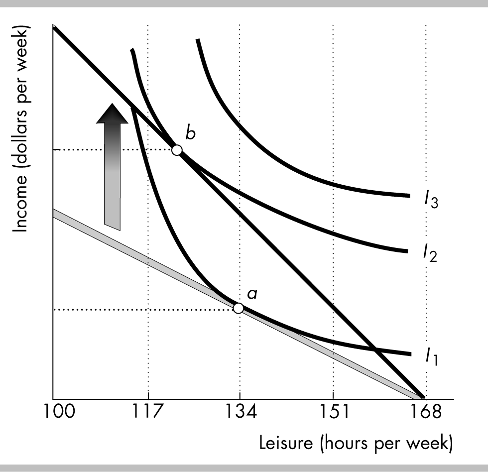
A household’s labor supply decisions can be analyzed using the same model of consumer choice. In this case, the two “goods” are leisure and income (from working). The income generated from working can then be used to purchase all other goods.
The household must allocate its time between leisure and work. The opportunity cost of an hour of leisure (that is, not working for an hour) is the wage rate.
 A
figure showing the indifference curves and the income-time budget
line is to the right. The maximum leisure is 168 hours a week, in
which case the person’s income is zero. The initial budget line is
the gray line.
A
figure showing the indifference curves and the income-time budget
line is to the right. The maximum leisure is 168 hours a week, in
which case the person’s income is zero. The initial budget line is
the gray line.
The person’s best affordable point is point a. The person has 134 hours of leisure a week, which means the person supplies 34 hours of labor a week.
An increase in the wage rate rotates the budget line upward, as shown in the figure. With the new, higher budget line, the person moves to the new best point, point b. At this point, the quantity of leisure consumed decreases, which means that the quantity of labor supplied increases.
The increase in the wage rate has a substitution effect and an income effect. The substitution effect occurs because an increase in the wage rate increases the opportunity cost of leisure, so people respond by substituting away from leisure. But the higher wage rate also increases the household’s income and the income effect leads to an increase in the demand for leisure, which is a normal good.
Between points a and b in the figure, the substitution effect dominates, so an increase in the wage rate increases the quantity of labor supplied. But if the wage rate increased more, so that the household could reach indifference curve I3, the income effect would dominate and the increase in wage rate would decrease the quantity of labor supplied.
Marginal Cost and Average Costs
Marginal cost (MC) is the increase in total cost that results from a one-unit increase in output. The MC curve is U-shaped.
Average fixed cost (AFC) is total fixed cost per unit of output. The value of AFC falls as output increases.
Average variable cost (AVC) is total variable costs per unit of output. At low levels of output, AVC falls as output increases but at higher levels of output, AVC rises as output increases.
Average total cost (ATC) is the total cost per unit of output. ATC = AFC + AVC. At low levels of output, ATC falls as output increases but at higher levels of output, ATC rises as output increases.
The figure illustrates typical MC, AFC, AVC, and ATC curves. As the figure shows, the MC curve, the AVC curve, and the ATC curve are all U-shaped. There are other additional important points about this figure:
T
 he
vertical distance between the AVC
curve and the ATC
curve is the AFC.
Because the AFC
decreases as output increases, these curves become vertically closer
to each other as output increases.
he
vertical distance between the AVC
curve and the ATC
curve is the AFC.
Because the AFC
decreases as output increases, these curves become vertically closer
to each other as output increases.The MC curve intersects the AVC curve and ATC curve at their minimums.
The shape of the cost curves is related to the shape of the productivity curves.
The shape of the AVC curve is determined by the shape of the AP curve. Over the range of output for which the AP curve is rising, the AVC curve is falling and over the range of output for which the AP curve is falling, the AVC curve is rising.
The shape of the MC curve is determined by the shape of the MP curve. Over the range of output for which the MP curve is rising, the MC curve is falling and over the range of output for which the MP curve is falling, the MC curve is rising.
The cost curves shift with changes in technology or changes in prices of factors of production.
An increase in technology that allows more output to be produced from the same resources shifts the
cost curves downward. If the technology requires more capital, a fixed input, then the average total cost curve shifts upward at low levels of output and downward at higher levels of output.
A fall in the price of the fixed factor shifts the AFC and ATC curves downward but leaves the AVC and MC curves unchanged. A fall in the price of a variable factor shifts the AVC, ATC, and MC curves downward but leaves the AFC curve unchanged.