Tangent-wedge method [from Anderson, 1989]

Instead of calculating the flowfield around the body itself, simple oblique shock theory can be applied to the constructed wedge shape to determine the desired properties at the point in question. This technique is known as the wedge or tangent-wedge method.

The conical flow, or tangent-cone, method is a similar idea in which the actual body is approximated as a cone-shaped axisymmetric body, as shown below. Thus, the properties at the point under consideration (i) can be obtained from conical flow tables for the correct Mach number.

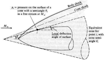
Tangent-cone method [from Anderson, 1989]

The wedge and cone methods are commonly used in hypersonic analysis methods because they are relatively simple but yield surprisingly accurate results. The conical flow technique is particularly popular and is frequently used to construct hypersonic flowfields from which waveriders are designed. A common variation on the technique is the osculating cones method in which multiple geometrically similar cones are employed. Each cone generates its own shock pattern and the conical shocks are merged together to generate a shock surface of constant strength. Thus, each cone is used to design a small section of the total flowfield.

Power Law methods:

During the 1960s, it became common practice to describe any hypersonic body of revolution using a parametric equation. The resulting shapes were referred to as power law bodies. Although power law equations can be used to define any shape, such as a wedge or cone, they are usually used to define optimum, minimum drag shapes. Power law bodies are typically defined by an equation of the form

where r = radial position, R = body radius, x = axial distance, l = body length, and m is an exponent typically between 0.5 and 0.8.

Many references refer to Ѕ power law bodies (i.e. m = 0.5) or ѕ power law bodies (i.e. m = 0.75), and waveriders have been designed using the known flowfields calculated for such bodies.

39. Pressure coefficient calculation by using Newtonian theory.

You can find many derivations of Newtonian theory on the internet or textbooks.

The derivation requires only knowledge of basic algebra and geometry.

The final results is a formula that relates the pressure coefficient, Cp,

Cp = 2cos2 (q )

The pressure at any given point on the body is dependent on only the incident free-stream direction.

Regions of the body on the leeward/shadow side (hidden from the free stream) are assumed to have a Cp =0

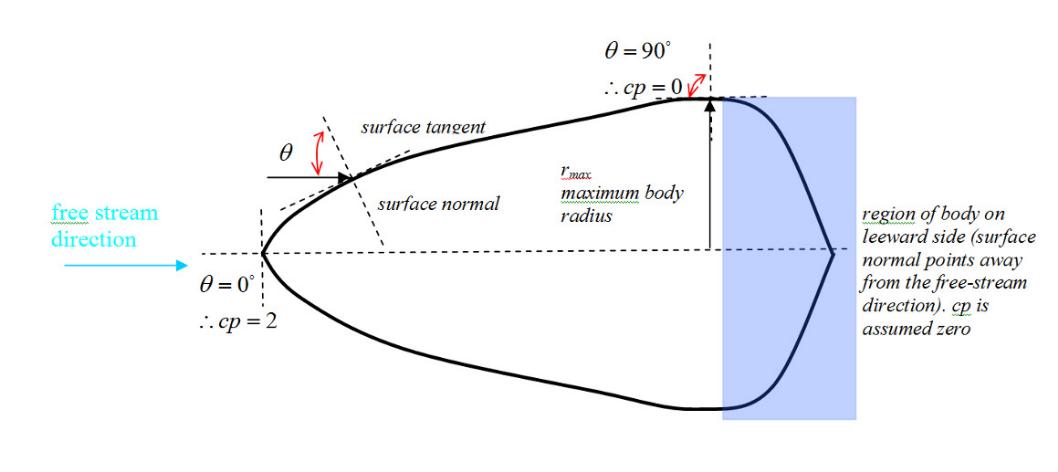
A bluff body in hypersonic flow showing surface normals. The region on the leeward side is shaded

The lift and drag can be found by integrating the Cp along the body surface.

The drag force is found from the Cp.

Often there is no simple analytical formula that describes the body for the calculation of normals and Cp.

The body surface must be divided into small regions and the normal and Cp calculated for each region.

40. What caloricaly perfect gas is? Can it be used for cflculation hypersonic flow?

Along with the definition of a perfect gas, there are also two more simplifications that can be made although various textbooks either omit or combine the following simplifications into a general "perfect gas" definition.

A thermally perfect gas

• is in thermodynamic equilibrium

• is not chemically reacting

• has internal energy e, enthalpy h, and specific heat C_V that are functions of temperature only and not of pressure, i.e., , , , .

This type of approximation is useful for modeling, for example, an axial compressor where temperature fluctuations are usually not large enough to cause any significant deviations from the thermally perfect gas model. Heat capacity is still allowed to vary, though only with temperature, and molecules are not permitted to dissociate. The latter implies temperature limited to 1500 K.^[2]

Even more restricted is the calorically perfect gas for which, in addition, the specific heat is assumed to be constant: and .

Although this may be the most restrictive model from a temperature perspective, it is accurate enough to make reasonable predictions within the limits specified. A comparison of calculations for one compression stage of an axial compressor (one with variable C_p, and one with constant C_p) produces a deviation small enough to support this approach. As it turns out, other factors come into play and dominate during this compression cycle. These other effects would have a greater impact on the final calculated result than whether or not C_p was held constan

41. Sense of the Newton’s model of fluid flow.

In continuum mechanics, a fluid is said to be Newtonian if the viscous stresses that arise from its flow, at every point, are proportional to the local strain rate — the rate of change of its deformation over time.^{[1] [2][3]} That is equivalent to saying that those forces are proportional to the rates of change of the fluid's velocity vector as one moves away from the point in question in various directions.

More precisely, a fluid is Newtonian if, and only if, the tensors that describe the viscous stress and the strain rate are related by a constant viscosity tensor that does not depend on the stress state and velocity of the flow. If the fluid is also isotropic (that is, its mechanical properties are the same along any direction), the viscosity tensor reduces to two real coefficients, describing the fluid's resistance to continuous shear deformation and continuous compression or expansion, respectively.

Newtonian fluids are the simplest mathematical models of fluids that account for viscosity. While no real fluid fits the definition perfectly, many common liquids and gases, such as water and air, can be assumed to be Newtonian for practical calculations under ordinary conditions. However, non-Newtonian fluids are relatively common, and include oobleck (which becomes stiffer when vigorously sheared), or non-drip paint (which becomes thinner when sheared). Other examples include many polymer solutions (which exhibit the Weissenberg effect), molten polymers, many solid suspensions, blood, and most highly viscous fluids.

An element of a flowing liquid or gas will suffer forces from the surrounding fluid, including viscous stress forces that cause it to gradually deform over time. These forces can be mathematically approximated to first order by a viscous stress tensor, which is usually denoted by .

The deformation of that fluid element, relative to some previous state, can be approximated to first order by a strain tensor that changes with time. The time derivative of that tensor is the strain rate tensor, that expresses how the element's deformation is changing with time; and is also the gradient of the velocity vector field at that point, often denoted .

The tensors and can be expressed by 3×3 matrices, relative to any chosen coordinate system. The fluid is said to be Newtonian if these matrices are related by the equation where is a fixed 3×3×3×3 fourth order tensor, that does not depend on the velocity or stress state of the fluid.