

32. Velocity field of rectangular horseshoe vortex (to write and explain or prove).
From
equation (2.12),
we define a horseshoe vortex as a line of constant strength lift
Oseenlets over a span s
such that L
is the total lift generated by the distribution. The lift Oseenlet is
given in terms of a potential velocity term ϕ
and a wake potential term Χ.
We investigate the velocity induced by each term in turn. Hence, we
consider![]() (3.1)
(3.1)
(a) Contribution from φ
We first
investigate the velocity induced by the potential velocity term φ,
which is given by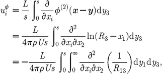 (3.2)where
![]() and
and
![]() ,
and where the identity
,
and where the identity![]() (3.3)has
been used;
(3.3)has
been used;
![]() .
This identity is used and proved in Chadwick
(2005).
.
This identity is used and proved in Chadwick
(2005).
Since the
Laplacian of 1/R
is zero for R>0
![]() ,
then we can rewrite equation (3.2)
as
,
then we can rewrite equation (3.2)
as (3.4)where
![]() for
for
![]() ,
(2, 3, 1) or (3, 1, 2),
,
(2, 3, 1) or (3, 1, 2),
![]() for
(i,
j,
q)=(1,
3, 2), (2, 1, 3) or (3, 2, 1), and
for
(i,
j,
q)=(1,
3, 2), (2, 1, 3) or (3, 2, 1), and
![]() otherwise.
As l≠2,
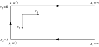
we can apply Stokes's theorem to get an integral over the horseshoe
vortex contour Ck
defined along the integral path consisting of the three straight
lines:
otherwise.
As l≠2,
we can apply Stokes's theorem to get an integral over the horseshoe
vortex contour Ck
defined along the integral path consisting of the three straight
lines:
![]() ;
;
![]() and
and
![]() (see
figure
1).
(see
figure
1).
View larger version:
In this page
In a new window
Download as PowerPoint Slide
Figure 1
Horseshoe contour.
Applying
Stokes's theorem and letting
![]() we
get
we
get![]() (3.5)where
the tangent vector in the anticlockwise sense, as represented in
figure
1,
is given by
(3.5)where
the tangent vector in the anticlockwise sense, as represented in
figure
1,
is given by
![]() .
This is the result for the potential part of the horseshoe vortex
given by equation (2.13).
.
This is the result for the potential part of the horseshoe vortex
given by equation (2.13).
(b) Contribution from Χ
Now consider
the contribution from the wake potential Χ.
This is given by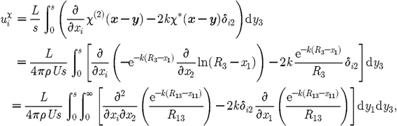 (3.6)where
we have let
(3.6)where
we have let
![]() .
However, Χ
satisfies
.
However, Χ
satisfies
![]() ,
and so
,
and so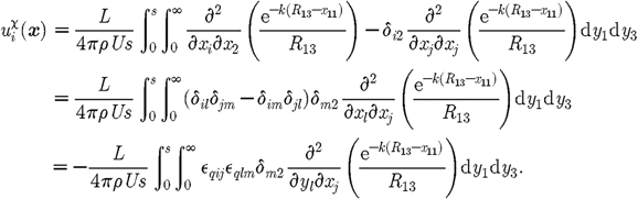 (3.7)Applying
Stokes's theorem and letting
we
get
(3.7)Applying
Stokes's theorem and letting
we
get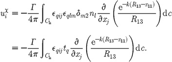 (3.8)
(3.8)
(c) The vortex line
Combining
equations (3.5)
and (3.8)
gives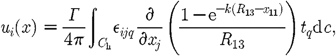 (3.9)which
is the result equation (2.13).
(3.9)which
is the result equation (2.13).
Consider the
arm of the trailing vortex line positioned from (0, 0, 0) to (∞, 0,
0). From equation (2.14)
this is given by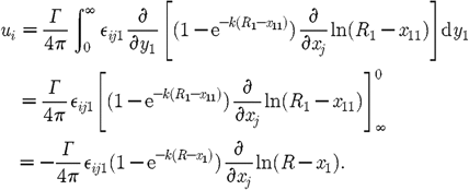 (3.10)
(d) The velocity near to the vortex line
We can use
this result to find the velocity near a vortex line. For small R−x1,
x1>0,
we have R−x1∼r2/2x1,
where
![]() ,
and so the velocity potential part of the vortex line is such
that
,
and so the velocity potential part of the vortex line is such
that![]() (3.11)where
(3.11)where
![]() is
the unit vector direction of the θ
cylindrical polar coordinate such that
is
the unit vector direction of the θ
cylindrical polar coordinate such that
![]() ,
,
![]() .
Hence the potential associated with this velocity is
.
Hence the potential associated with this velocity is
![]() ,
near to the vortex line, which is the inviscid result. Similarly, the
velocity near the vortex line is given by
,
near to the vortex line, which is the inviscid result. Similarly, the
velocity near the vortex line is given by![]() (3.12)which
in the plane of constant x1
gives the core radius
(3.12)which
in the plane of constant x1
gives the core radius
![]() ,
and yields the Lamb–Oseen vortex (Delbende
et
al.
2004)
,
and yields the Lamb–Oseen vortex (Delbende
et
al.
2004)![]() (3.13)Batchelor
(1964)
demonstrates that the solution given by equation (3.12)
yields a pressure deficit. However, from the horseshoe vortex
description equation (3.9),
this deficit is implicitly accounted for by the inclusion of the
axial velocity term generated by the bound vortex line
(3.13)Batchelor
(1964)
demonstrates that the solution given by equation (3.12)
yields a pressure deficit. However, from the horseshoe vortex
description equation (3.9),
this deficit is implicitly accounted for by the inclusion of the
axial velocity term generated by the bound vortex line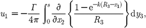 (3.14)which
then means that the Bernoulli equation is satisfied to first order.
To first order this is
(3.14)which
then means that the Bernoulli equation is satisfied to first order.
To first order this is
![]() which
is also the Oseen pressure equation. Seeking an asymptotic form of
equation (3.14),
gives
which
is also the Oseen pressure equation. Seeking an asymptotic form of
equation (3.14),
gives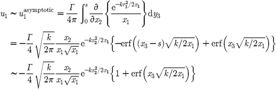 (3.15)as
s→∞,
where the function erf is the error function (Abramowitz
& Stegun 1965).
This solution (3.15)
is antisymmetric in x2.
This is to be expected for a solution related to the generation of
lift in the x2
direction. This is also to be expected as the Oseen solution is a
linearization of the velocity, and so can be represented by a
distribution of Oseenlet solutions generated by the potentials φ,
Χ
and Χ*.
Hence, given the symmetry of the velocity in the transverse plane, it
is possible to infer the symmetry in the streamwise direction. This
suggests that, for the streamwise velocity, any functions of x2
and x3
are odd. In contrast, Batchelor seeks a term symmetric in x2
and x3
to satisfy the pressure imbalance given by the Bernouilli equation.
This yields an entirely different solution, which to leading order
is
(3.15)as
s→∞,
where the function erf is the error function (Abramowitz
& Stegun 1965).
This solution (3.15)
is antisymmetric in x2.
This is to be expected for a solution related to the generation of
lift in the x2
direction. This is also to be expected as the Oseen solution is a
linearization of the velocity, and so can be represented by a
distribution of Oseenlet solutions generated by the potentials φ,
Χ
and Χ*.
Hence, given the symmetry of the velocity in the transverse plane, it
is possible to infer the symmetry in the streamwise direction. This
suggests that, for the streamwise velocity, any functions of x2
and x3
are odd. In contrast, Batchelor seeks a term symmetric in x2
and x3
to satisfy the pressure imbalance given by the Bernouilli equation.
This yields an entirely different solution, which to leading order
is![]() (3.16)for
some constant A.
If Batchelor had sought an antisymmetric solution in x2
instead, then the solution (3.15)
rather than (3.16)
would have been obtained. We suggest that for flow past a body that
can be represented by the horseshoe vortex model, then equation
(3.14)
is the appropriate streamwise component to balance pressure and
equation (3.15)
is the appropriate near vortex asymptotic approximation.
(3.16)for
some constant A.
If Batchelor had sought an antisymmetric solution in x2
instead, then the solution (3.15)
rather than (3.16)
would have been obtained. We suggest that for flow past a body that
can be represented by the horseshoe vortex model, then equation
(3.14)
is the appropriate streamwise component to balance pressure and
equation (3.15)
is the appropriate near vortex asymptotic approximation.
Furthermore,
as streamlines separate from the generating body (for example, wing
tip) at the boundary of the vortex core, there must also be a
potential outflow which can only be produced by a streamwise drag
Oseenlet in the Oseen flow formulation. This gives an additional
streamwise velocity component, which reduces to![]() (3.17)near
to the vortex line, where D
is the drag. Assuming x1
is again to first order constant this reduces to the Batchelor vortex
representation in the plane of constant x1,
or q-vortex
(Delbende
et
al.
2004)
such that
(3.17)near
to the vortex line, where D
is the drag. Assuming x1
is again to first order constant this reduces to the Batchelor vortex
representation in the plane of constant x1,
or q-vortex
(Delbende
et
al.
2004)
such that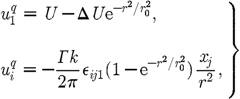 (3.18)for
some constant ΔU.
Taking a further approximation to equation (3.12),
gives
(3.18)for
some constant ΔU.
Taking a further approximation to equation (3.12),
gives![]() (3.19)Hence,
in the eye of the vortex line, the fluid velocity is finite and is
the uniform stream velocity to first order.
(3.19)Hence,
in the eye of the vortex line, the fluid velocity is finite and is
the uniform stream velocity to first order.
Previous SectionNext Section
4. The far field wake
Consider the
force
![]() ,
then the far field velocity is given by
,
then the far field velocity is given by![]() (4.1)
(4.1)
(a) Flow near to wake line
Close to the
wake line,![]() (4.2)and
so
(4.2)and
so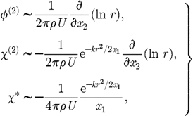 (4.3)which
is the far field laminar wake solution of Landau
& Liftshitz (1959,
pp. 74–75) near to the wake line. This solution is also the
three-dimensional extension of the two-dimensional result from
boundary layer theory for flow past a flat plate (Katz
& Plotkin 2001,
p. 472; Schlichting
1979,
p. 177). Hence, in the far field wake, boundary layer flow and Oseen
flow give the same solution. Furthermore, we see a relation for the
near field flows of the vortex line and the lift Oseenlet: The lift
Oseenlet flow is the same as the flow obtained in the limit as the
span of the horseshoe vortex tends to zero: In other words,
(4.3)which
is the far field laminar wake solution of Landau
& Liftshitz (1959,
pp. 74–75) near to the wake line. This solution is also the
three-dimensional extension of the two-dimensional result from
boundary layer theory for flow past a flat plate (Katz
& Plotkin 2001,
p. 472; Schlichting
1979,
p. 177). Hence, in the far field wake, boundary layer flow and Oseen
flow give the same solution. Furthermore, we see a relation for the
near field flows of the vortex line and the lift Oseenlet: The lift
Oseenlet flow is the same as the flow obtained in the limit as the
span of the horseshoe vortex tends to zero: In other words,
![]() and
and
![]() in
the near field. This relation between the lift Oseenlet and horseshoe
vortex for the potential velocity is given in Chadwick
(2005).
in
the near field. This relation between the lift Oseenlet and horseshoe
vortex for the potential velocity is given in Chadwick
(2005).
(b) Flow far from wake line
Far from the
wake line, the vortex wake potential Χ
is negligible. So Χ(2)∼0,
Χ*∼0
and![]() (4.4)In
spherical polars
(4.4)In
spherical polars
![]() ,
,
![]() ,
,
![]() ,
then
,
then![]() (4.5)Similarly,
Χ(1)∼0,
and
(4.5)Similarly,
Χ(1)∼0,
and![]() (4.6)which
is the far field laminar wake solution of Landau and Lifshitz (Landau
& Liftshitz 1959,
p. 76) away from the wake line.
(4.6)which
is the far field laminar wake solution of Landau and Lifshitz (Landau
& Liftshitz 1959,
p. 76) away from the wake line.
33. Sense (idea) of calculation unsteady aerodynamic performances (forces), using vortex lattice numerical method for two dimensional flow.
The synthesis of a comprehensive theory of force production in insect flight is hindered in part by the lack of precise knowledge of unsteady forces produced by wings. Data are especially sparse in the intermediate Reynolds number regime (10<Re<1000) appropriate for the flight of small insects. This paper attempts to fill this deficit by quantifying the time-dependence of aerodynamic forces for a simple yet important motion, rapid acceleration from rest to a constant velocity at a fixed angle of attack. The study couples the measurement of lift and drag on a two-dimensional model with simultaneous flow visualization. The results of these experiments are summarized below. 1. At angles of attack below 13.5°, there was virtually no evidence of a delay in the generation of lift, in contrast to similar studies made at higher Reynolds numbers. 2. At angles of attack above 13.5°, impulsive movement resulted in the production of a leading edge vortex that stayed attached to the wing for the first 2 chord lengths of travel, resulting in an 80 % increase in lift compared to the performance measured 5 chord lengths later. It is argued that this increase is due to the process of detached vortex lift, analogous to the method of force production in delta-wing aircraft. 3. As the initial leading edge vortex is shed from the wing, a second vortex of opposite vorticity develops from the trailing edge of the wing, correlating with a decrease in lift production. This pattern of alternating leading and trailing edge vortices generates a von Karman street, which is stable for at least 7.5 chord lengths of travel. 4. Throughout the first 7.5 chords of travel the model wing exhibits a broad lift plateau at angles of attack up to 54°, which is not significantly altered by the addition of wing camber or surface projections. 5. Taken together, these results indicate how the unsteady process of vortex generation at large angles of attack might contribute to the production of aerodynamic forces in insect flight. Because the fly wing typically moves only 2–4 chord lengths each half-stroke, the complex dynamic behavior of impulsively started wing profiles is more appropriate for models of insect flight than are steady-state approximations.
34. To write the formulas for calculation aerodynamic coefficients of the airfoil cross-section in linear case.
Coefficient
may also be used as a characteristic of a particular shape (or
cross-section) of an airfoil.
In this application it is called the section
lift coefficient
![]() It
is common to show, for a particular airfoil section, the relationship
between section lift coefficient and angle
of attack.[5]
It is also useful to show the relationship between section lift
coefficient and drag
coefficient.
It
is common to show, for a particular airfoil section, the relationship
between section lift coefficient and angle
of attack.[5]
It is also useful to show the relationship between section lift
coefficient and drag
coefficient.
The section lift coefficient is
based on two-dimensional flow over a wing of infinite span and
non-varying cross-section so the lift is independent of spanwise
effects and is defined in terms of
![]() ,
the lift force per unit span of the wing. The definition becomes
,
the lift force per unit span of the wing. The definition becomes
![]() ,
,
where
![]() is
the chord
of the airfoil.
is
the chord
of the airfoil.
For a given angle of attack cl can be calculated approximately using the thin airfoil theory,[6] calculated numerically or determined from wind tunnel tests on a finite-length test piece, with end-plates designed to ameliorate the three-dimensional effects. Plots of cl versus angle of attack show the same general shape for all airfoils, but the particular numbers will vary. They show an almost linear increase in lift coefficient with increasing angle of attack with a gradient known as the lift slope. For a thin airfoil of any shape the lift slope is π2/90 ≃ 0.11 per degree. At higher angles a maximum point is reached, after which the lift coefficient reduces. The angle at which maximum lift coefficient occurs is the stall angle of the airfoil.
Symmetric airfoils necessarily have plots of cl versus angle of attack symmetric about the cl axis but for any airfoil with positive camber, i.e. asymmetrical, convex from above, there is still a small but positive lift coefficient with angles of attack less than zero. That is, the angle at which cl=0 is negative. On such airfoils at zero angle of attack the pressures on the upper surface are lower than on the lower surface
35. Aerodynamic hysteresis, what is it?
Hysteresis is the dependence of a system not only on its current environment but also on its past environment. This dependence arises because the system can be in more than one internal state. To predict its future development, either its internal state or its history must be known.[1] If a given input alternately increases and decreases, the output tends to form a loop as in the figure. However, loops may also occur because of a dynamic lag between input and output. Often, this effect is also referred to as hysteresis, or rate-dependent hysteresis. However, this effect disappears as the input changes more slowly.
Hysteresis occurs in ferromagnetic materials and ferroelectric materials, as well as in the deformation of some materials (such as rubber bands and shape-memory alloys) in response to a varying force. In natural systems hysteresis is often associated with irreversible thermodynamic change. Many artificial systems are designed to have hysteresis: for example, in thermostats and Schmitt triggers, hysteresis is used to avoid unwanted rapid switching. Hysteresis has been identified in many other fields, including economics and biology.
In aerodynamics, hysteresis can be observed when decreasing the angle of attack of a wing after stall, regarding the lift and drag coefficients. The angle of attack where the flow on top of the wing reattaches is generally lower than the angle of attack where the flow separates during the increase of the angle of attack.[7]
36. To write the formula for calculation velocity, induced by the segment of the straight line vortex.
The velocityfield of a straight vortex segment serves as a simple illustration of the application of Biot-Savart’s law. However, it is also a very useful result since the numericalsolutionof more complicated geometries canbe obtainedbydiscretizing thevortex sheetinto a lattice of straight concentrated vortex elements. The result to be derived here therefore serves as the influence function for such a computational scheme.
We can simplify the analysisby choosinga coordinate system such that thevortexsegment coincides with thex axis and the fieldpoint,P, lies on theyaxis, as shownin figure 48. This is not really a restriction, since one can always make a coordinatetransformationtodothis,andtheresultingvelocity vectorcanthenbe transformedback to the original global coordinate system.
The vortex extends along the x axis from x1 to x2. In this case
~s =(1, 0, 0) and ~r =(−ξ,y, 0)
and from equation 104 we can see immediately that u = v = 0, so that we only need to develop the expression for w,
w(y)=4Γ π Zxx12 (ξ2 +ydξ y2)3/2 =4πy Γ "√ξ2 ξ+y2 #x2 =4πy Γ _xb2 −xc1 _ (106)
x1
Where b = x22 +y2 and c = x21 +y2 . This result can alsobe expressed in terms of the two angles θ1 and θ2 which are illustrated in figure 48,
w(y)=4πy[cos θ2 +cosθ1]
37. Qualitative aspects of hypersonic flow.
In aerodynamics, a hypersonic speed is one that is highly supersonic (even though the origin of the words is the same: "super" is the Latin cognate of the Greek "hyper"). Since the 1970s, the term has generally been assumed to refer to speeds of Mach 5 and above.
The precise Mach number at which a craft can be said to be flying at hypersonic speed varies, since individual physical changes in the airflow (like molecular dissociation and ionization) occur at different speeds; these effects collectively become important around Mach 5. The hypersonic regime is often alternatively defined as speeds where ramjets do not produce net thrust.
While the definition of hypersonic flow can be quite vague and is generally debatable (especially due to the lack of discontinuity between supersonic and hypersonic flows), a hypersonic flow may be characterized by certain physical phenomena that can no longer be analytically discounted as in supersonic flow. The peculiarity in hypersonic flows are as follows:
Shock layer
Aerodynamic heating
Entropy layer
Real gas effects
Low density effects
Independence of aerodynamic coefficients with Mach number.
38. Newtonian theory application for hypersonic flow.