

Determination of critical rotational speeds taking into account
Influence of gyroscopic moment
When determining critical rotational speed above only centrifugal forces of unbalanced weights were considered. In some cases, as it was shown, precession of the shaft causes gyroscopic moment appearance, which can largely change the value of rotor critical rotational speed.
The sag y and angle of section turn in the point of concentrated force Рс and gyroscopic (bending) moment MG action (Fig. 8.15) (under the principle of independence of forces action on elastic systems) can be presented as follows:
![]() (8.9)
(8.9)
where y1P is a sag caused by the force Р=1; y1M is a sag caused by the moment М=1; 1P is a turn angle caused by the force Р=1; 1M is a turn angle caused by the moment М=1.

Fig. 8.15. For determination of rotor critical rotational speed taking into account
gyroscopic moment influence
The centrifugal force of disc inertia and gyroscopic moment, appearing when the shaft rotates, are respectively equal to:
![]() (8.10)
(8.10)
Substituting values Рс and МG in equations (8.9), we will get two equations with two unknown quantities:
![]()
We solve these equations regarding y and :
 (8.11)
If the denominator of these expressions is equal to zero, the sag y and turn angle show unlimited increase, that corresponds to shaft critical angular velocity cr. Therefore, equation
![]() (8.12)
(8.12)
is the requirement for determination of shaft critical angular velocity with one disc taking into account gyroscopic moment. Solving this biquadratic equation, it is easy to determine the value cr.
The
unit displacements
![]() ,
called influence
coefficients,
are determined with the help of Mohr’s
formulas
(known
from materials strength course):
,
called influence
coefficients,
are determined with the help of Mohr’s
formulas
(known
from materials strength course):
 (8.13)
where
![]() are the bending momenta in shaft sections caused by force Р=1
and bending moment М=1,
respectively.
are the bending momenta in shaft sections caused by force Р=1
and bending moment М=1,
respectively.
The
equality
![]() follows from the theorem
of reciprocity of single elastic displacements.
follows from the theorem
of reciprocity of single elastic displacements.
As
it’s known, Vereshchagin’s
rule
is the easiest way to calculate integrals in formulas
(8.13).According to this rule the
bending moment diagrams
![]() and
and
![]() are constructed, which are located one under another. The shaft is
segmented, within the limits of which, its flexural stiffness Е1
is constant, and the diagrams
and
have no changes of direction. After that, for each segment, one
diagram area is multiplied by the other diagram ordinate under the
centre of area weight of the first diagram. The multiplication
results are divided by rigidity of the congruent segments, and then
are summed up.
are constructed, which are located one under another. The shaft is
segmented, within the limits of which, its flexural stiffness Е1
is constant, and the diagrams
and
have no changes of direction. After that, for each segment, one
diagram area is multiplied by the other diagram ordinate under the
centre of area weight of the first diagram. The multiplication
results are divided by rigidity of the congruent segments, and then
are summed up.
Let us consider the scheme of calculation taking variable rigidity shaft as an example (Fig. 8.16).
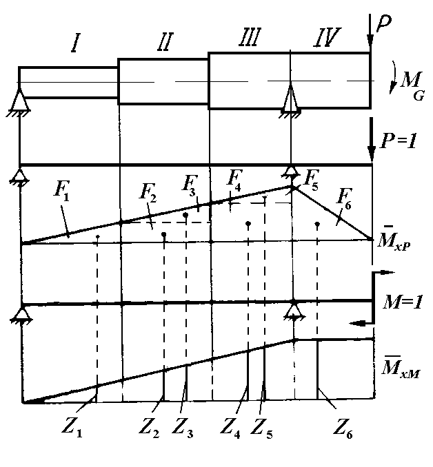
Fig. 8.16. To determine of value with the help of Vereshchagin’s rule
The shaft is divided into four segments – I, II, III, IV. Division of shaft part, with rigidity EI3, into two segments (III and IV) is caused by the fact that both diagrams ( and ) have changes of direction in support point.
Multiplying the areas of segments by the congruent ordinates under Vereshchagin’s rule, we will get:
![]() (8.14)
(8.14)
where F1, F2…F6 are the segments areas of the bending moment diagram caused by a single force action (of first diagram); z1, z2…z6 are ordinates of the bending moment diagram caused by a single moment action and taken under the centre of area weight of the first diagram.
Segmentation of the area within the limits of segments II and III is made for comfortable definition of diagram centre of area weight.
Values
![]() and
and
![]() are determined in a similar way but in these cases one diagram can
be constructed instead of two, then multiplying its segments areas by
the congruent ordinates of diagram centres of areas weight
(Fig. 8.17).
are determined in a similar way but in these cases one diagram can
be constructed instead of two, then multiplying its segments areas by
the congruent ordinates of diagram centres of areas weight
(Fig. 8.17).
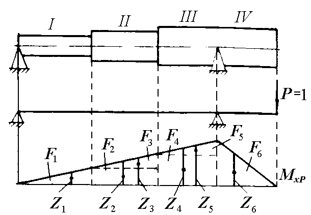
Fig. 8.17. To determine value with the help of Vereshchagin’s rule
The influence coefficients for the shaft with constant cross section at the different schemes of disc arrangement are shown in Tab. 8.1.
In
case of a direct precession (at
![]() )
the equation (8.12) has the only one real positive root cr1,
)
the equation (8.12) has the only one real positive root cr1,
In
case of retrograde precession (at
![]() )
the equation (8.12) has two real positive roots cr2
and cr3,
the values of which essentially differ from each other, with cr2
less, and cr3
more than critical rotational speed cr1
at
direct precession.
)
the equation (8.12) has two real positive roots cr2
and cr3,
the values of which essentially differ from each other, with cr2
less, and cr3
more than critical rotational speed cr1
at
direct precession.