2.2 Centrifugal pump characteristics

Centrifugal pumps are generally characterized by:

• most common and most preferred for pipeline applications

• minimal discharge pulsation

• capability of efficient performance over a wide range of pressure and capacities requirement for most pipeline applications)

• capability of high and variable throughputs

• discharge pressure and hence head are mostly a function of fluid density

• relatively small devices are less costly than other types of pumps

• high reliability

• can be used with viscosities up to 300 centipoise (cP), depending on pump size and speed before efficiency losses begin to be economically significant

• can be multi-staged for higher heads

Typical pipeline centrifugal pumps are shown in Fig. 2-3.

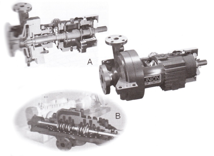
Figure 2-3. Typical Pipeline Centrifugal Single (A) and Multistage (B) pumps

Centrifugal Pump Performance Curves. An individual set of pump performance с is derived from a "family" set of pump curves, as illustrated in Fig. 2-4. The following information can usually be obtained:

• pump model and size

• rated speed

• curve identification number

• impeller type and eye area

• wear ring clearances

• range of impeller diameters available

• capacity versus head developed for the different impeller diameters (H-Q curves),

• power to drive pump (pressure head, flow P-Q) curves, based on water, specific gravity (SG= 1.0)

• pump efficiency (efficiency - Q curves)

• NPSHR

• pump specific speed, N_s

• pump suction specific speed, N_ss or S

Figure 2-4. Typical Centrifugal Multistage pump performance curve, m-pump 3x6 MOF-S5 stage

In a double suction pump, the area of the impeller eye is the area of the impeller eyes in both of the impellers. Pump shutoff is the head developed at zero (0) capacity. Pump run­out is the pump capacity above which the pump should not be operated due to instability, excessive NPSHR, vibration, and a dramatic reduction in head. This point is usually 120% of best efficiency point.

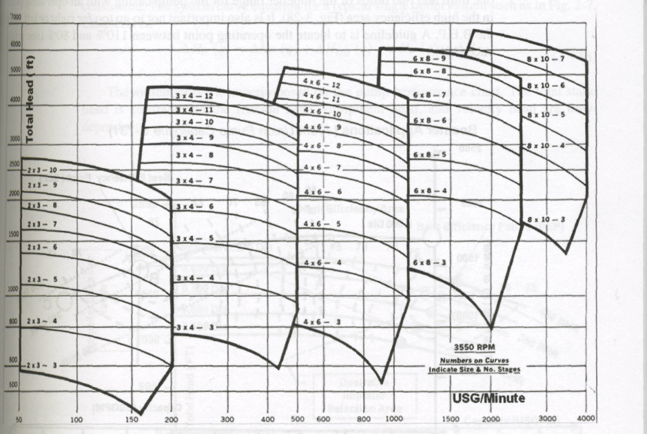
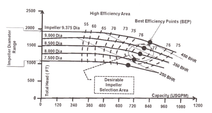
Centrifugal Pumps Coverage Chart. A coverage chart makes it possible to do a pre­liminary pump assessment and, hence, selection by reviewing a wide range of pump cas­ing/impeller sizes for a specific impeller speed. This chart helps narrow down the choice of pumps that will satisfy the pipeline system requirements. A typical pump selection chart is indicated in Fig. 2-5.

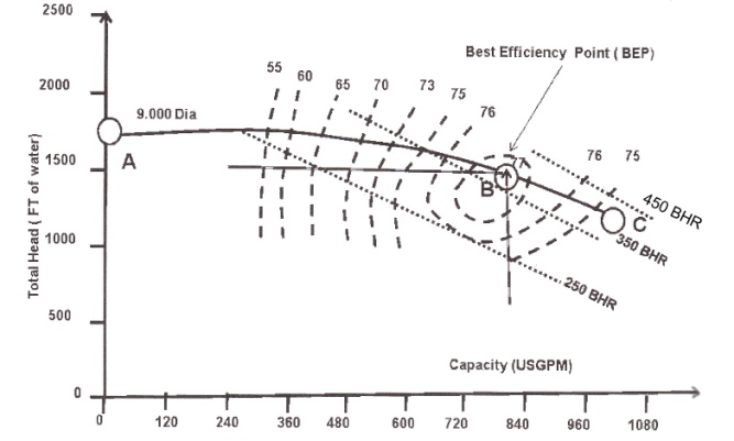
In selecting a pump to match the system curve, a pump with the appropriate impeller diameter must be selected to assure meeting the flow and head requirements. Determination of system total head for a given flow rate will determine pump selection based on pump performance curve for a given impeller diameter. As an example, Fig. 2-6 indicate the per­formance curve for a system operation with a pump that has an impeller diameter of 9" in.

Figure 2-5. Typical Range Of Multistage Centrifugal Pumps For Pipeline Booster Applications (from Union Pumps Catalogue C-731)

A performance curve plot commences at zero flow. The head at this point corresponds to the shutoff head of the pump, point A in Fig. 2-6. Starting at this point, the head decreases until it reaches its minimum at point B. This point is sometimes called the run-out point and represents the maximum flow of the pump. Beyond this, the pump cannot operate. The pump's range of operation is from points A to B.

Figure 2- 6. Typical performance curve for a specific 81/2’’ diameter impeller

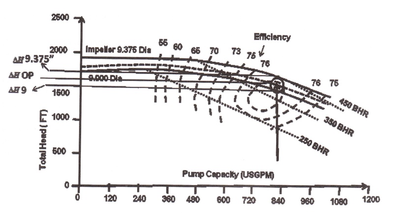
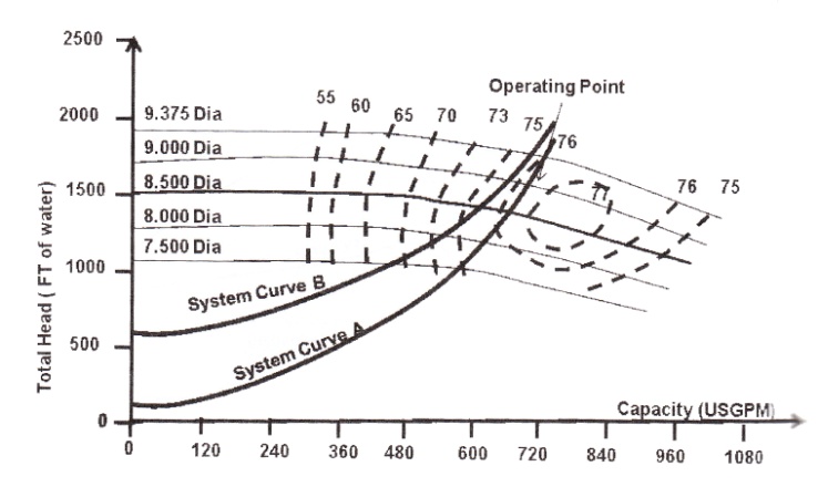
Impeller Selection. Quite often, the operating point is located between two curvesB a given performance chart.

The required impeller size can be calculated by the linear interpolation of adjacent B curve that fall above and below the operating point, in this case 9- and 9.375-in. impeller sizes (Fig. 2-7). The following equation will give the correct size:

, (2-1)

where

D_OP - impeller diameter required

ΔH_op = pump total head at the operating point

ΔH₉ = pump total head at the intersection of the 9 in. impeller curve and flow rate

ΔH_9.375 = pump total head at the intersection of the 9.375 in. impeller curve and flow rate

Figure 2-7. Desirable pump selection area

When possible, a pump is selected with an impeller that can be increased in size,] mitting a future increase in head and capacity or, alternatively, an impeller which cat reduced in size. As a guide, select a pump with an impeller size no greater than between one third and two thirds of the impeller range for the pump casing with an operating роint in the high efficiency area (Fig. 2-8). It is also important not to go too far right or left from the B.E.P. A guideline is to locate the operating point between 110% and 80% (see reference [16]).

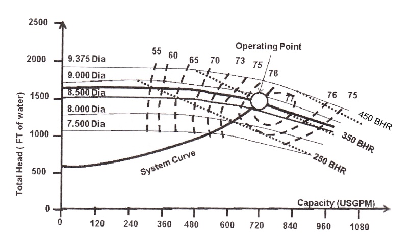
Pump Head-Flow and System Head Flow Curves. The system curve is a plot of the total head versus the flow for a given system.

The higher the flow, the greater the head required (Fig. 2-9). The shape of the system curve depends on the type of system being considered. The system curve equation for a typical single outlet system such as in Fig. 2-7, Chapter 2 is:

, (2-2)

The system curve is superimposed on the pump performance chart. The total static head is constant and the friction head, equipment head, and velocity head are flow-dependent.

Figure 2-8. Desirable pump selection area

The calculation of total head at different flow rates produces a plot of total head versus flow, thus producing the system curve.

The operating point is the point on the system curve corresponding to the flow end head required. It is also the point where the system curve intersects the period curve.

Figure 2-9. Pump performance- system curve superimposition

The design system curve is usually calculated with extra flow capacity in mind. As usually the demand changes towards higher deliveries, it is good practice to plot the system curve for higher flow rates than the design flow rate. Thus, unanticipated extra capacity can be accommodated if required.

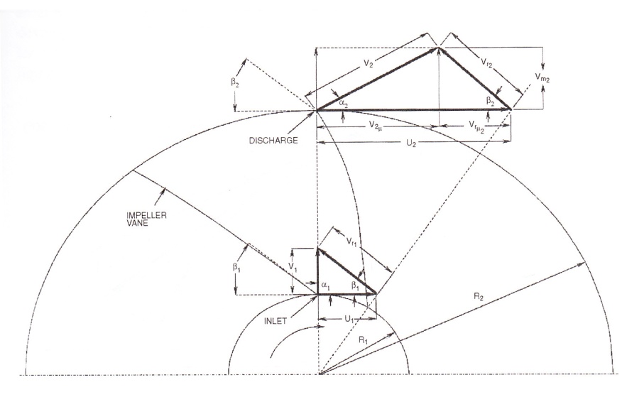
Centrifugal Impeller Design Theory. The work of a centrifugal impeller (H_t) can be derived by applying the principle of angular momentum to the mass of fluid going through the impeller passages. This principle is applied to the inlet and exit conditions of a friction less fluid in an impeller to drive the impeller head H_t

Using the following nomenclature:

U = peripheral velocity of impeller

V_r = relative velocity of flow

V = absolute velocity of flow

V_m = radial velocity

α,β =vane angle

ω = angular velocity

γ = density

g = gravitational acceleration

Q = flow

W = weight flow

1. = inlet subscript

2. = discharge subscript

Figure 2-10 depicts a sketch of an impeller inlet and discharge velocity diagram.

The torque (T) is defined as the difference of the peripheral components of impulse forces:

, (2-3)

, (2-4)

, (2-5)

Considering Euler’s theory the following can be derived for the work done by the impeller (i.e., theoretical head H_t achieved):

, (2-6)

’ (2-7)

Substituting:

, (2-8)

Figure 2-10. Impeller inlet and discharge velocity diagram

The Euler Equation for head H_t is thus:

, (2-9)

Assuming the fluid enters the impeller without a tangential component (radial inlet) then V_1u U₁=0 and Euler’s Eq. (2-9) can be reduced to:

, (2-10)

, (2-11)

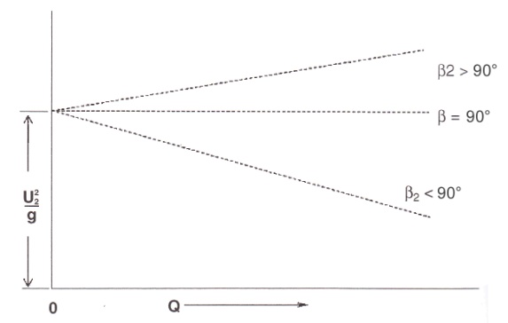
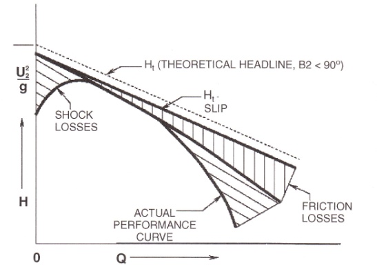
For any given impeller size, V_m2 will vary directly with flow, and if the rotative speed is held constant, U₂ will be constant and H_t will vary linearly with flow. For an angle β₂ less than 90° (backward curved vanes), VmVtan /3₂ will increase with flow and cause H_fto decrease with flow. This will result in a theoretical curve, as shown in Fig. 3-31. If shock losses, slip factors and friction losses are added to the theoretical curve, the typical pump characteristic curve (as shown in Fig. 2-11) is generated. It is these types of curves that pipeline engineers need to be familiar with in order to select pumps for a particular service application.

Figure 2-11. Development of the pump head capacity curve

Specific Speed. Generally, there are a multitude of pipeline pump designs that are avail­able for any given task including for pipeline applications. Pump users generally would like to know the pump performance for their applications and, hence, what efficiency can be expected from a particular pump design.

For pump performance comparison purposes, pumps are tested and compared using various criteria including and, importantly, the criterion of specific speed (NS). The ef­ficiency of pumps with the same specific speed can be compared providing the user or the designer a starting point for comparison or as a benchmark for improving the design and increasing the efficiency.

Specific speed (N_s) is thus used to predict pump characteristics for the purpose of clas­sifying pump impellers according to type, proportions and performance. It is expressed as:

, (2-12)

where

N_s = pump specific speed (dimensionless)

N - pump speed in RPM

Q = capacity at best efficiency point (USGPM)

H = total head per stage at the best efficiency point (ft)

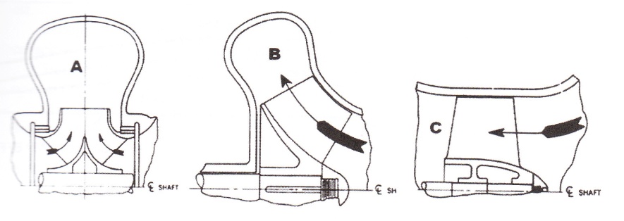
Centrifugal pumps are traditionally divided into 3 types: radial flow, mixed flow, and axial flow (Fig. 2-12). There is a continuous change from the radial flow impeller, which develops pressure principally from the action of centrifugal force, to the axial flow impel­ler, which develops most of its head by the propelling or lifting action of the vanes on the liquid.

Figure 2-12. Centrifugal Pump Cross Sections, A: Radial Flow, B: Mixed Flow & C: Axial Flow

The above equation is for single suction pumps. For double suction impellers, one half the flow needs to be used to calculate the specific speed. The specific speed (N) determines the general shape or class of the impeller. As the specific speed increases, the ratio oil impeller outlet diameter, D₂, to the inlet or eye diameter, £>,, decreases. This ratio becomes 1.0 for a true axial flow impeller.

Radial flow impellers develop head mainly through centrifugal force. Pumps of Me specific speeds develop head partially by centrifugal force and partially by axial force. A pump with a higher specific speed generates head more by axial forces and less by centrifugal forces. An axial flow or propeller pump with a specific speed of 10,000 or greater generates its head exclusively through axial forces.

The specific speed of an impeller can thus provide a wide variety of information the performance:

• Impeller type: impellers with low specific speed are long and thin and are used for low flow, high head applications. Impellers with high specific speed are short and stubby are used for high-flow, low-head applications.

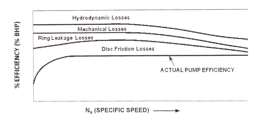
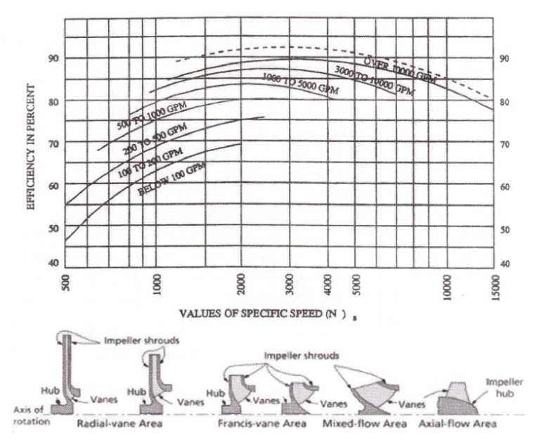
• Efficiency: efficiency is arrived at by considering the losses through the pump impeller and driver system. Pump efficiency is affected by losses due to pump impeller friction, ring leakage, and mechanical losses as well as losses incurred by movement of the liquid within the pump, referred to as hydrodynamic losses. Specific speed affects pump efficiency (Fig. 2-13). The lower the specific speed, the lower the efficiency. The reason is that a higher percentage of energy is lost to overcome the impeller disc friction that is necessary to generate the high heads (Fig. 2-14).

Figure 2-13. Specific speed and efficiency

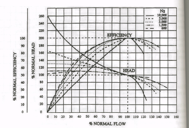
• Shape of curve: once an impeller is designed for a certain specific speed, it will produce a typical head capacity curve and efficiency curve shape. A low specific speed impeller has a flat curve with a wide efficiency range. A high specific speed impeller produces a steep curve with a narrow efficiency range (Fig. 2-15).

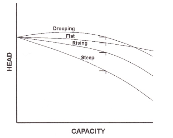
Impeller Curve Characteristics. There are a number of pump head capacity (H-QI curve shapes that are shown in Fig. 2-16. These characteristic curves are listed below and described thereafter:

• rising

• drooping

• steep

• flat

• stable

• unstable

• non-overloading

• overloading

Figure 2-14. Specific speed and efficiency (R. Darby, 1996 Courtesy Chemical Engineering Fluid Mechanics, Marcel Dekker)

Rising characteristic: the head rises continuously as the capacity is decreased to shut-off.

Drooping characteristic: the head developed at shut-off is less than at some of the other capacities.

Steep characteristic: the head developed at shutoff is significantly larger than that devel­oped at the design capacity.

Flat characteristic: the head developed at shut-off is approximately that developed at the design capacity. The curve can be a slightly rising or drooping.

Stable curve: is a rising curve where only one capacity can be obtained at any one head. A curve with a rising characteristic would be an example of a stable curve.

Unstable curve: is a drooping curve where more than one capacity can be obtained at one head. A curve with a drooping characteristic would be an example of an unstable curve.

Figure 2-15. Specific speed and performance

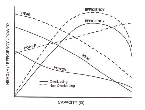
Non-overloading curve (Fig. 2-17): power curve continues to increase with an increase in capacity.

Overloading curve (Fig. 2-17): power curve continues to decrease with an increase in capacity.

Affinity Laws. The flow and head of a centrifugal pump may be changed by varying the I pump speed or changing the impeller diameter. This results in a change to the impeller tip I speed or velocity of the impeller vanes, which causes a change in the velocity at which the I liquid leaves the impeller. Usually, the impellers can be cut down to 80% of the original I diameter without lowering the efficiency significantly.

The affinity laws were developed using the laws of similitudes which provides three I basic relationships

• Flow versus diameter

• Total head versus diameter and speed

• Power versus diameter and speed

Figure 2-16. Various types of pump characteristic curves

For centrifugal pumps with radial impellers the relationships are approximately as follows:

For diameter change only:

, (2-13)

Figure 2-17. Typical characteristic curves for overloading and non-overloading

For speed change only:

, (2-14)

For diameter and speed change:

, (2-15)

Where

D = impeller diameter (typically in inches)

H = head in (typically in feet or meter)

Q = capacity (typically in USGPM)

N = speed in RPM

bhp = brake horsepower

1. = original conditions subscript

2. = new design conditions subscript

The process of arriving at the affinity laws assumes that the two operating points that are being compared are at the same efficiency. The relationship between two operate points, say 1 and 2, depends on the shape of the system curve (Fig. 2-18).

Figure 2-18. Limitation on the use of the affinity laws

The points that lie on system curve A will all be approximately at the same efficiency, whereas the points that lie on system curve В are not. The affinity laws do not apply to points that belong to system curve B. System curve В describes a system with a relatively high static head vs. system curve A, which has a low static head [8].

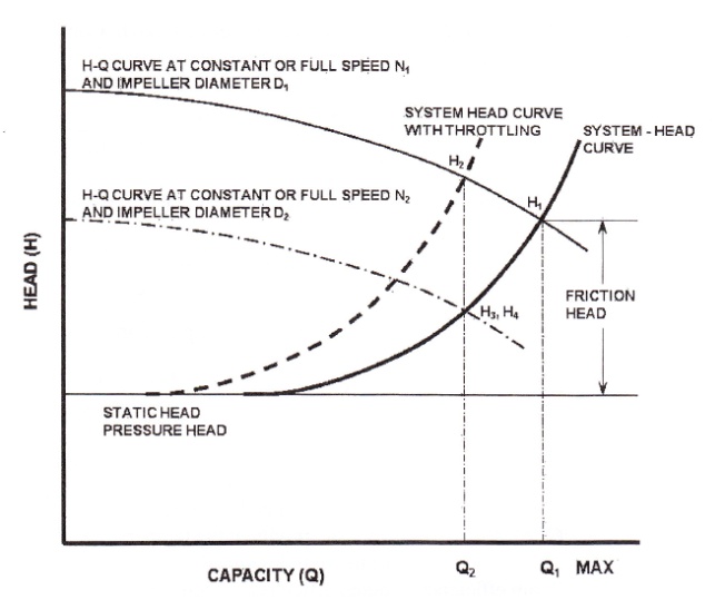
Pipeline-Pump Operational Control (Pump Head-Flow and System Head-Flow Curves. Pumps and pipelines can be controlled by several means including pressure/flow throttling through the appropriate suction/discharge valves, speed changes, etc. To illustrate these options, a pump H-Q curve overlaid on the pipeline system hydraulic system head curve is shown in Fig. 2-19.

In this example, the pump is designed to operate at point Я, unless the pump or the system curve is changed.

The pump includes a throttle valve on the discharge side. If such a throttle valve is partially closed, friction will be added to the system and the pump is forced to operate back on the curve at Point H_r When the system head curve is changed by throttling, it is called "throttle control."

If the speed of the pump is reduced from N_{ to N₂ or the impeller decliner is reduced from D₁ to D₂, then the H-Q curve is changed, as shown in Fig. 2-19. The pump would now operate at point H₃ (for speed reduction) or H₄ (for diameter change).

Figure 2-19. Capacity change with throttling

Pump Sizing and Selection. When sizing and selecting centrifugal pumps, it is most economical to use the physically smallest pump that will perform the service. Pumps are sized on the following basis:

• Suction and discharge nozzles. Suction nozzles are the same size or larger than the of the discharge nozzles. The discharge nozzle is never larger than the suction nozzle. The larger the nozzle size the higher the flow capacity of the pump.

• Impeller diameter. The larger the impeller diameter, the higher the head (and hence the discharge pressure). The head is proportional to the square of the impeller di­ameter. However, due to the effect of inertia (stresses caused by centrifugal force), impeller size is limited by speed. Typical speeds are 1800 RPM for 26-in. impeller and 3600 RPM for 12-in. impeller chambers.

• Speed. The flow rate varies linearly with speed, the head varies as the square and the power varies as the cube of the speed change. Centrifugal pumps are generally not used below 1200 RPM because of the low head developed.

• Suction limitations. The suction conditions quite often are the limiting factors that affect speed, size, and capacity. Requirements are determined by the NPSHR, which will be defined later in this chapter.

Centrifugal Pump Power and Efficiency. Brake horsepower is the actual power delivered to the pump shaft. It is expressed as

, (2-16)

Hydraulic horsepower is the liquid power delivered by the pump. It is expressed as:

Centrifugal Pump Power and Efficiency. Brake horsepower is the actual poweril ered to the pump shaft. It is expressed as:

, (2-17)

The pump efficiency is the ratio of hyd hp and bhp:

, (2-18)

Where

Q = flow capacity (USGPM)

H = total developed head (feet)

G = specific gravity at the temperature of the liquid pumped

Pump efficiency = pump efficiency in percent (%)