The Heckscher-Ohlin (Factor Proportions) Model

Note: This page provides an overview of the Heckscher-Ohlin model assumptions and results. To find out more details about each issue, click on the MORE INFO links scattered on the page.

The factor proportions model was originally developed by two Swedish economists, Eli Heckscher and his student Bertil Ohlin in the 1920s. Many elaborations of the model were provided by Paul Samuelson after the 1930s and thus sometimes the model is referred to as the Heckscher-Ohlin-Samuelson (or HOS) model. In the 1950s and 60s some noteworthy extensions to the model were made by Jaroslav Vanek and so occasionally the model is called the Heckscher-Ohlin-Vanek model. Here we will simply call all versions of the model either the "Heckscher-Ohlin (or H-O) model" or simply the more generic "factor-proportions model".

The H-O model incorporates a number of realistic characteristics of production that are left out of the simple Ricardian model. Recall that in the simple Ricardian model only one factor of production, labor, is needed to produce goods and services. The productivity of labor is assumed to vary across countries which implies a difference in technology between nations. It was the difference in technology that motivated advantageous international trade in the model.

The standard H-O model⁽¹⁾ begins by expanding the number of factors of production from one to two. The model assumes that labor and capital are used in the production of two final goods. Here, capital refers to the physical machines and equipment that is used in production. Thus, machine tools, conveyers, trucks, forklifts, computers, office buildings, office supplies, and much more, is considered capital.

All productive capital must be owned by someone. In a capitalist economy most of the physical capital is owned by individuals and businesses. In a socialist economy productive capital would be owned by the government. In most economies today, the government owns some of the productive capital but private citizens and businesses own most of the capital. Any person who owns common stock issued by a business has an ownership share in that company and is entitled to dividends or income based on the profitability of the company. As such, that person is a capitalist, i.e., an owner of capital.

The H-O model assumes private ownership of capital. Use of capital in production will generate income for the owner. We will refer to that income as capital "rents". Thus, whereas the worker earns "wages" for their efforts in production, the capital owner earns rents.

The assumption of two productive factors, capital and labor, allows for the introduction of another realistic feature in production; that of differing factor-proportions both across and within industries. When one considers a range of industries in a country it is easy to convince oneself that the proportion of capital to labor used varies considerably. For example, steel production generally involves large amounts of expensive machines and equipment spread over perhaps hundreds of acres of land, but also uses relatively few workers. In the tomato industry, in contrast, harvesting requires hundreds of migrant workers to hand-pick and collect each fruit from the vine. The amount of machinery used in this process is relatively small.

In the H-O model we define the ratio of the quantity of capital to the quantity of labor used in a production process as the capital-labor ratio. We imagine, and therefore assume, that different industries, producing different goods, have different capital-labor ratios. It is this ratio (or proportion) of one factor to another that gives the model its generic name: the factor-proportions model.

In a model in which each country produces two goods, an assumption must be made as to which industry has the larger capital-labor ratio. Thus, if the two goods that a country can produce are steel and clothing, and if steel production uses more capital per unit of labor than is used in clothing production, then we would say the steel production is capital-intensive relative to clothing production. Also, if steel production is capital-intensive, then it implies that clothing production must be labor-intensive relative to steel. MORE INFO

Another realistic characteristic of the world is that countries have different quantities, or endowments, of capital and labor available for use in the production process. Thus, some countries like the US are well-endowed with physical capital relative to its labor force. In contrast many less developed countries have very little physical capital but are well-endowed with large labor forces. We use the ratio of the aggregate endowment of capital to the aggregate endowment of labor to define relative factor abundancy between countries. Thus if, for example, the US has a larger ratio of aggregate capital per unit of labor than France's ratio, we would say that the US is capital-abundant relative to France. By implication, France would have a larger ratio of aggregate labor per unit of capital and thus France would be labor-abundant relative to the US. MORE INFO

The H-O model assumes that the only difference between countries is these differences in the relative endowments of factors of production. It is ultimately shown that trade will occur, trade will be nationally advantageous, and trade will have characterizable effects upon prices, wages and rents, when the nations differ in their relative factor endowments and when different industries use factors in different proportions.

It is worth emphasizing here a fundamental distinction between the H-O model and the Ricardian model. Whereas the Ricardian model assumes that production technologies differ between countries, the H-O model assumes that production technologies are the same. The reason for the identical technology assumption in the H-O model is perhaps not so much because it is believed that technologies are really the same; although a case can be made for that. Instead the assumption is useful because it enables us to see precisely how differences in resource endowments is sufficient to cause trade and it shows what impacts will arise entirely due to these differences.

The Main Results of the H-O Model

There are four main theorems in the H-O model; the Heckscher-Ohlin theorem, the Stolper-Samuelson Theorem, the Rybczynski theorem, and the factor-price equalization theorem. The Stolper-Samuelson and Rybczynski theorems describe relationships between variables in the model while the H-O and factor-price equalization theorems present some of the key results of the model. Applications of these theorems also allows us to derive some other important implications of the model. Let us begin with the H-O theorem.

The Heckscher-Ohlin Theorem

The H-O theorem predicts the pattern of trade between countries based on the characteristics of the countries. The H-O theorem says that a capital-abundant country will export the capital-intensive good while the labor-abundant country will export the labor-intensive good.

Here's why.

A capital-abundant country is one that is well-endowed with capital relative to the other country. This gives the country a propensity for producing the good which uses relatively more capital in the production process, i.e., the capital-intensive good. As a result, if these two countries were not trading initially, i.e., they were in autarky, the price of the capital-intensive good in the capital-abundant country would be bid down (due to its extra supply) relative to the price of the good in the other country. Similarly, in the labor-abundant country the price of the labor-intensive good would be bid down relative to the price of that good in the capital-abundant country.

Once trade is allowed, profit-seeking firms will move their products to the markets that temporarily have the higher price. Thus the capital-abundant country will export the capital-intensive good since the price will be temporarily higher in the other country. Likewise the labor-abundant country will export the labor-intensive good. Trade flows will rise until the price of both goods are equalized in the two markets.

The H-O theorem demonstrates that differences in resource endowments as defined by national abundancies is one reason that international trade may occur. MORE INFO

The Stolper-Samuelson Theorem

The Stolper-Samuelson theorem describes the relationship between changes in output, or goods, prices and changes in factor prices such as wages and rents within the context of the H-O model. The theorem was originally developed to illuminate the issue of how tariffs would affect the incomes of workers and capitalists (i.e., the distribution of income) within a country. However, the theorem is just as useful when applied to trade liberalization.

The theorem states that if the price of the capital-intensive good rises (for whatever reason) then the price of capital, the factor used intensively in that industry, will rise, while the wage rate paid to labor will fall. Thus, if the price of steel were to rise, and if steel were capital-intensive, then the rental rate on capital would rise while the wage rate would fall. Similarly, if the price of the labor-intensive good were to rise then the wage rate would rise while the rental rate would fall. MORE INFO

The theorem was later generalized by Jones who constructed a magnification effect for prices in the context of the H-O model. The magnification effect allows for analysis of any change in the prices of the both goods and provides information about the magnitude of the effects on the wages and rents. Most importantly, the magnification effect allows one to analyze the effects of price changes on real wages and real rents earned by workers and capital owners. This is instructive since real returns indicate the purchasing power of wages and rents after accounting for the price changes and thus are a better measure of well-being than simply the wage rate or rental rate alone. MORE INFO

Since prices change in a country when trade liberalization occurs, the magnification effect can be applied to yield an interesting and important result. A movement to free trade will cause the real return of a country's relatively abundant factor to rise, while the real return of the country's relatively scarce factor will fall. Thus if the US and France are two countries who move to free trade, and if the US is capital-abundant (while France is labor-abundant) then capital owners in the US will experience an increase in the purchasing power of their rental income (i.e., they will gain) while workers will experience a decline in the purchasing power of their wage income (i.e., they will lose). Similarly, workers will gain in France, but capital owners will lose.

What's more the country's abundant factor benefits, regardless in which industry it is employed. Thus, capital owners in the US would benefit from trade even if their capital is used in the declining import-competing sector. Similarly, workers would lose in the US even if they are employed in the expanding export sector.

The reasons for this result are somewhat complicated but the gist can be given fairly easily. When a country moves to free trade the price of its exported goods will rise while the price of its imported goods will fall. The higher prices in the export industry will inspire profit-seeking firms to expand production. At the same time, in the import-competing industry suffering from falling prices, will want to reduce production to cut their losses. Thus, capital and labor will be laid-off in the import-competing sector but will be in demand in the expanding export sector. However, a problem arises in that the export sector is intensive in the country's abundant factor, let's say capital. This means that the export industry wants relatively more capital per worker than the ratio of factors that the import-competing industry is laying off. In the transition there will be an excess demand for capital, which will bid up its price, and an excess supply of labor, which will bid down its price. Hence, the capital owners in both industries experience an increase in their rents while the workers in both industries experiences a decline in their wages.

The Factor-Price Equalization Theorem

The factor-price equalization theorem says that when the prices of the output goods are equalized between countries, as when countries move to free trade, then the prices of the factors (capital and labor) will also be equalized between countries. This implies that free trade will equalize the wages of workers and the rentals earned on capital throughout the world.

The theorem derives from the assumptions of the model, the most critical of which is the assumption that the two countries share the same production technology and that markets are perfectly competitive. In a perfectly competitive market factors are paid on the basis of the value of their marginal productivity which in turn depends upon the output prices of the goods. Thus, when prices differ between countries so will their marginal productivities and hence so will their wages and rents. However, once goods prices are equalized, as they are in free trade, the value of marginal products are also equalized between countries and hence the countries must also share the same wage rates and rental rates.

Factor-price equalization formed the basis for some arguments often heard in the debates leading up to the approval of the North American Free Trade Agreement (NAFTA) between the US, Canada and Mexico. Opponents of NAFTA feared that free trade with Mexico would lower US wages to the level in Mexico. Factor-price equalization is consistent with this fear although a more likely outcome would be a reduction in US wages coupled with an increase in Mexican wages.

Furthermore, we should note that the factor-price equalization is unlikely to apply perfectly in the real world. The H-O model assumes that technology is the same between countries in order to focus on the effects of different factor endowments. If production technologies differ across countries, as we assumed in the Ricardian model, then factor prices would not equalize once goods prices equalize. As such a better interpretation of the factor-price equalization theorem applied to real world settings is that free trade should cause a tendency for factor prices to move together if some of the trade between countries is based on differences in factor endowments. MORE INFO

The Rybczynski Theorem

The Rybczynski theorem demonstrates the relationship between changes in national factor endowments and changes in the outputs of the final goods within the context of the H-O model. Briefly stated it says that an increase in a country's endowment of a factor will cause an increase in output of the good which uses that factor intensively, and a decrease in the output of the other good. In other words if the US experiences an increase in capital equipment, then that would cause an increase in output of the capital-intensive good, steel, and a decrease in the output of the labor-intensive good, clothing. The theorem is useful in addressing issues such as investment, population growth and hence labor force growth, immigration and emigration, all within the context of the H-O model. MORE INFO

The theorem was also generalized by Jones who constructed a magnification effect for quantities in the context of the H-O model. The magnification effect allows for analysis of any change in both endowments and provides information about the magnitude of the effects on the outputs of the two goods. MORE INFO

Aggregate Economic Efficiency

The H-O model demonstrates that when countries move to free trade, they will experience an increase in aggregate efficiency. The change in prices will cause a shift in production of both goods in both countries. Each country will produce more of its export good and less of its import goods. Unlike the Ricardian model, however, neither country will necessarily specialize in production of its export good. As a result of the production shifts though, productive efficiency in each country will improve. Also, due to the changes in prices, consumers, in the aggregate will experience an improvement in consumption efficiency. In other words, national welfare will rise for both countries when they move to free trade. MORE INFO

However, this does not imply that everyone benefits. As was discussed above, the model clearly shows that some factor owners will experience an increase in their real incomes while others will experience a decrease in their factor incomes. Trade will generate winners and losers. The increase in national welfare essentially means that the sum of the gains to the winners will exceed the sum of the losses to the losers. For this reason economists often apply the compensation principle.

The compensation principle states that as long as the total benefits exceed the total losses in the movement to free trade, then it must be possible to redistribute income from the winners to the losers such that everyone has at least as much as they had before trade liberalization occurred. MORE INFO

1. The "standard" H-O model refers to the case of two countries, two goods and two factors of production. The H-O model has been extended to a many country, many goods and many factors case but most of the exposition in this text, and by economists in general, is in reference to the standard case.

Heckscher-Ohlin Model Assumptions

Perfect Competition prevails in all markets.

Two countries

The case of two countries is used to simplify the model analysis. Let one country be the US, the other France*. Note, anything related exclusively to France* in the model will be marked with an asterisk.

Two goods

Two goods are produced by both countries. We assume a barter economy. This means that there is no money used to make transactions. Instead, for trade to occur, goods must be traded for other goods. Thus we need at least two goods in the model. Let the two produced goods be clothing and steel.

Two factors

Two factors of production, labor and capital, are used to produce clothing and steel. Both labor and capital are homogeneous. Thus there is only one type of labor and one type of capital. The laborers and capital equipment in different industries are exactly the same. We also assume that labor and capital are freely mobile across industries within the country but immobile across countries. Free mobility makes the H-O model a long-run model.

Factor Constraints

The total amount of labor and capital used in production is limited to the endowment of the country.

The Labor Constraint is,

where and are the quantities of labor used in clothing and steel production, respectively. L represents the labor endowment of the country. Full employment of labor implies the expression would hold with equality.

The Capital Constraint is,

where and are the quantities of capital used in clothing and steel production, respectively. K represents the capital endowment of the country. Full employment of capital implies the expression would hold with equality.

Endowments

The only difference between countries assumed in the model is differences in endowments of capital and labor.

Definition

A country is capital abundant relative to another country if it has more capital endowment per labor endowment than the other country. Thus in this model the US is capital abundant relative to France if:

where K is the capital endowment, L the labor endowment in the US. K* is the capital endowment, L* the labor endowment in France.

Note that if the US is capital abundant then France is labor abundant since the above inequality can be rewritten to get:

This means that France has more labor per unit of capital for use in production than the US.

Demand

Factor owners are the consumers of the goods. The factor owners have a well defined utility function defined over the two goods. Consumers maximize utility to allocate income between the two goods.

When necessary we will assume that aggregate preferences can be represented by a homothetic utility function of the form where C_S is the amount of steel consumed and C_C is the amount of clothing consumed.

General Equilibrium

The H-O model is a general equilibrium model. The income earned by the factors is used to purchase the two goods. The industries' revenue in turn is used to pay for the factor services. The prices of outputs and factors in an equilibrium are those which equalize supply and demand in all markets simultaneously.

Heckscher-Ohlin Model Assumptions – Production

The production functions below represent industry production not firm production. The industry consists of many small firms in light of the assumption of perfect competition.

Production of Clothing

US	France

where

Q_C = quantity of clothing produced in the US measured in racks.

L_C = amount of labor applied to clothing production in the US measured in labor-hours.

K_C = amount of capital applied to clothing production in the US measured in capital-hours.

f( ) = the clothing production function which transforms labor and capital inputs into clothing output.

and where all starred variables are defined in the same way but refer to the production process in France.

Production of Steel

US	France

where

Q_S = quantity of steel produced in the US measured in tons.

L_S = amount of labor applied to steel production in the US measured in labor-hours.

K_S = amount of capital applied to steel production in the US measured in capital-hours.

g( ) = the steel production function which transforms labor and capital inputs into steel output.

and where all starred variables are defined in the same way but refer to the production process in France.

Production functions are assumed to be identical across countries within an industry. Thus both the US and France share the same production function f(.) for clothing and g(.) for steel. This means that the countries share the same technologies. Neither country has a technological advantage over the other. This is different from the Ricardian model which assumed that technologies were different across countries.

A simple formulation of the production process is possible by defining the unit-factor requirements.

Let,

represent the unit-labor requirement in clothing production.

It is the number of labor-hours needed to produce a rack of clothing.

Let,

represent the unit-capital requirement in clothing production.

It is the number of capital-hours needed to produce a rack of clothing.

Similarly,

is the unit-labor requirement in steel production.

It is the number of labor-hours needed to produce a ton of steel.

And,

is the unit-capital requirement in steel production.

It is the number of capital-hours needed to produce a ton of steel.

By taking the ratios of the unit-factor requirements in each industry we can define a capital-labor (or labor-capital) ratio. These ratios, one for each industry, represent the proportions in which factors are used in the production process. They are also the basis for the model's name.

First, is the capital-labor ratio in clothing production. It is the proportion in which capital and labor are used to produce clothing.

Similarly is the capital-labor ratio in steel production. It is the proportion in which capital and labor are used to produce steel.

Definition

We say that steel production is capital intensive relative to clothing production if:

This means steel production requires more capital per labor-hour than is required in clothing production.

Notice that if steel is capital intensive, clothing must be labor intensive.

Clothing production is labor intensive relative to steel production if:

This means clothing production requires more labor per capital-hour than steel production.

REMEMBER

Factor Intensity is a comparison of production processes across industries but within a country.

Factor Abundancy is a comparison of endowments across countries.

Heckscher-Ohlin Model Assumptions: Fixed versus Variable Proportions

Two different assumptions can be applied in a Heckscher-Ohlin model, fixed and variable proportions. A fixed proportions assumption means that the capital-labor ratio in each production process is fixed. A variable proportions assumption means that the capital-labor ratio can adjust to changes in the wage rate for labor and rental rate for capital.

Fixed proportions is a more simplistic and also less realistic assumption. However, many of the primary results of the H-O model can be demonstrated within the context of fixed proportions. Thus the fixed proportions assumption is useful in deriving the fundamental theorems of the H-O model. The variable proportions assumption is more realistic but makes solving the model significantly more difficult analytically. To derive the theorems of the H-O model under variable proportions often requires the use of calculus.

Fixed Factor Proportions

Fixed factor proportions means that a_KC, a_LC, a_KS, and a_LS are exogenous to the model and are fixed. Since the capital-output and labor-output ratios are fixed, the capital-labor ratios, and , are also fixed. Thus, clothing production must use capital to labor in a particular proportion regardless of the quantity of clothing produced. The ratio of capital to labor used in steel production is also fixed but is assumed different from the proportion used in clothing production.

Variable Factor Proportions

Under variable proportions the capital-labor ratio used in the production process is endogenous. The ratio will vary with changes in the factor prices. Thus if there were a large increase in wage rates paid to labor, producers would reduce their demand for labor and substitute relatively cheaper capital in the production process. This means a_KC and a_LC are variable rather than fixed. So as the wage and rental rates change, the capital output ratio and the labor output ratio are also going to change.

The Production Possibility Frontier (Fixed Proportions Case)

The production possibility frontier can be derived in the fixed proportions case by using the exogenous factor requirements to rewrite the labor and capital constraints. The labor constraint with full employment can be written as,

The capital constraint with full employment becomes,

Each of these constraint contains two endogenous variables Q_C and Q_S. The remaining variables are exogenous.

We graph the two constraints in the adjoining Figure.

The red line is the labor constraint. The endpoints and represent the maximum quantities of clothing and steel that could be produced if all of the labor endowment were allocated to clothing and steel production, respectively. All points on the line represent combinations of clothing and steel output which could employ all of the labor available in the economy. Points outside the constraint, such as B and D, are not feasible production points since there is insufficient labor resources. All points on or within the line, such as A, C and E, are feasible. The slope of the labor constraint is .

The blue line is the capital constraint. The endpoints and represent the maximum quantities of clothing and steel that could be produced if all of the capital endowment were allocated to clothing and steel production, respectively. Points on the line represent combinations of clothing and steel production which would employ all of the capital in the economy. Points outside the constraint, such as A and D, are not feasible production points since there is insufficient capital resources. Points on or within the line, such as B, C and E, are feasible. The slope of the capital constraint is .

The production possibility frontier is the set of output combinations which generate full employment of resources - in this case both labor and capital. Only one point, point E, can simultaneously generate full employment of both labor and capital. Thus point E is the PPF. The production possibility set is the set of all output combinations that are feasible. The PPS is the area bounded be the axes and the interior section of the labor and capital constraints. Thus at points like A there is sufficient labor to make production feasible but insufficient capital, thus point A is not a feasible production point. Similarly, at point B there is sufficient capital but not enough labor. Points like C however, which lie inside (or on) both factor constraints do represent feasible production points.

Note that the labor constraint is drawn with a steeper slope than the capital constraint. This implies, which in turn implies (with cross multiplication), . This means that steel is assumed to be capital intensive and clothing production is labor-intensive. If the slope of the capital constraint had been steeper then the factor intensities would be reversed.

The Rybczynski Theorem

The Relationship between Endowments and Outputs.

The Rybczynski theorem demonstrates how changes in an endowment affects the outputs of the goods when full employment is maintained. The theorem is useful in analyzing the effects of capital investment, immigration and emigration within the context of a H-O model. Consider a diagram depicting a labor constraint in red (it's the steeper lower line) and a capital constraint in blue (the flatter line). Suppose production occurs initially on the PPF at point A.

Next, suppose there is an increase in the labor endowment. This will cause an outward parallel shift in the labor constraint. The PPF and thus production will shift to point B. Production of clothing, the labor intensive good, will rise from C1 to C2. Production of steel, the capital-intensive good, will fall from S1 to S2.

If the endowment of capital rose the capital constraint would shift out causing an increase in steel production and a decrease in clothing production. Recall that since the labor constraint is steeper than the capital constraint, steel is capital-intensive and clothing is labor-intensive.

This means that in general, an increase in a country's endowment of a factor will cause an increase in output of the good which uses that factor intensively, and a decrease in the output of the other good.

The Magnification Effect for Quantities

The magnification effect for quantities is a more general version of the Rybczynski theorem. It allows for changes in both endowments simultaneously and allows a comparison of the magnitudes of the changes in endowments and outputs.

The simplest way to derive the magnification effect is with a numerical example.

Suppose the exogenous variables of the model take the following values for one country:

With these numbers which means that steel production is capital-intensive and clothing is labor-intensive.

The labor and capital constraints are,

Labor Constraint:

Capital Constraint:

We graph these on the adjacent Figure. The steeper red line is the labor constraint, the flatter blue line, the capital constraint. The output quantities on the PPF can be found by solving

the two constraint equations simultaneously.

A simple method to solve these equations follows.

First, multiply the second equation by (-2) to get,

Adding these two equations vertically yields,

which implies, . Plugging this into the first equation above (any equation will do) yields, . Simplifying we get, .

Thus, the solution to the two equations is: Q_C = 24 and Q_S = 24

Next suppose the capital endowment, K, increases to 150. This changes the capital constraint but leaves the labor constraint unchanged. The labor and capital constraints now are,

Labor Constraint:

Capital Constraint:

Follow the same procedure to solve for the outputs in the new full employment equilibrium.

First, multiply the second equation by (-2) to get,

Adding these two equations vertically yields,

which implies, . Plugging this into the first equation above (any equation will do) yields, . Simplifying we get, .

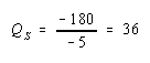
Thus the new solution is: Q_C = 6 and Q_S = 36.

The Rybczynski theorem says that if the capital endowment rises it will cause an increase in output of the capital intensive good (in this case steel) and a decrease in output of the labor intensive good (clothing). In this numerical example Q_S rises from 24 to 36, Q_C falls from 24 to 6.

The magnification effect for quantities ranks the percentage changes in endowments and the percentage changes in outputs. We'll denote the percentage change by using a ^ above the variable. (that is, = % change in X).

Percentage Changes in the Endowments and Outputs

The capital stock rises by 25%.

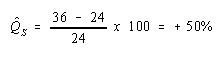
The quantity of steel rises by 50%.

The quantity of clothing falls by 75%.

The labor stock is unchanged.

The rank order of these changes is the Magnification Effect for Quantities,

The effect is initiated by changes in the endowments. If the endowments change by some percentages, ordered as above, then the quantity of the capital-intensive good (steel) will rise by a larger percentage than the capital stock change. The size of the effect is magnified relative to the cause.

The quantity of cloth (Q_C) changes by a smaller percentage than the smaller labor endowment change. Its effect is magnified downward.

Although this effect was derived only for the specific numerical values assumed in the example, it is possible to show, using more advanced methods, that the effect will arise for any endowment changes that are made. Thus if the labor endowment were to rise with no change in the capital endowment, the magnification effect would be,

This implies that the quantity of the labor-intensive good (clothing) would rise by a greater percentage than the quantity of labor, while the quantity of steel would fall.

The magnification effect for quantities is a generalization of the Rybczynski theorem. The effect allows for changes in both endowments simultaneously and provides information about the magnitude of the effects. The Rybczynski theorem is one special case of the magnification effect assuming one of the endowments is held fixed.

Although the magnification effect is shown here under the special assumption of fixed factor proportions and for a particular set of parameter values, the result is much more general. It is possible, using calculus, to show that the effect is valid under any set of parameter values and in a more general variable proportions model.

The Magnification Effect for Prices

The magnification effect for prices is a more general version of the Stolper-Samuelson theorem. It allows for simultaneous changes in both output prices and compares the magnitudes of the changes in output and factor prices.

The simplest way to derive the magnification effect is with a numerical example.

Suppose the exogenous variables of the model take the following values for one country:

		PS = 120
		PC = 40

With these numbers which means that steel production is capital-intensive and clothing is labor-intensive.

The zero-profit conditions in the two industries are,

Zero-profit Steel:

Zero-profit Clothing:

The equilibrium wage and rental rates can be found by solving the two constraint equations simultaneously.

A simple method to solve these equations follows.

First, multiply the second equation by (-4) to get,

Adding these two equations vertically yields,

which implies, . Plugging this into the first equation above (any equation will do) yields, . Simplifying we get, .

Thus the initial equilibrium wage and rental rates are: w = 8 and r = 24.

Next suppose the price of clothing, P_C, rises from $40 to $60 per rack. This changes the zero-profit condition in clothing production but leaves the zero-profit condition in steel unchanged. The zero-profit conditions now are,

Zero-profit Steel:

Zero-profit Clothing:

Follow the same procedure to solve for the equilibrium wage and rental rates.

First, multiply the second equation by (-4) to get,

Adding these two equations vertically yields,

which implies, . Plugging this into the first equation above (any equation will do) yields, . Simplifying we get, .

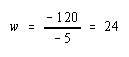
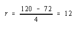
Thus the new equilibrium wage and rental rates are: w = 24 and r = 12.

The Stolper-Samuelson theorem says that if the price of clothing rises, it will cause an increase in the price paid to the factor used intensively in clothing production (in this case the wage rate to labor) and a decrease in the price of the other factor (the rental rate on capital). In this numerical example w rises from $8 to $24 per hour, r falls from $24 to $12 per hour.

The magnification effect for prices ranks the percentage changes in output prices and the percentage changes in factor prices. We'll denote the percentage change by using a ^ above the variable. (that is, = % change in X).

Percentage Changes in the Goods and Factor Prices

The price of clothing rises by 50%.

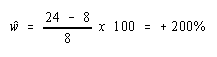The wage rate rises by 200%.

The rental rate falls by 50%.

The price of steel is unchanged

The rank order of these changes is the Magnification Effect for Prices,

The effect is initiated by changes in the output prices. These appear in the middle of the inequality. If output prices change by some percentages, ordered as above, then the wage rate paid to labor will rise by a larger percentage than the price of steel changes. The size of the effect is magnified relative to the cause.

The rental rate changes by a smaller percentage than the price of steel changes. Its effect is magnified downward.

Although this effect was derived only for the specific numerical values assumed in the example, it is possible to show, using more advanced methods, that the effect will arise for any output price changes that are made. Thus if the price of steel were to rise with no change in the price of clothing, the magnification effect would be,

This implies that the rental rate would rise by a greater percentage than the price of steel, while the wage rate would fall.

The magnification effect for prices is a generalization of the Stolper-Samuelson theorem. The effect allows for changes in both output prices simultaneously and provides information about the magnitude of the effects. The Stolper-Samuelson theorem is a special case of the magnification effect when one of the endowments is held fixed.

Although the magnification effect is shown here under the special assumption of fixed factor proportions and for a particular set of parameter values, the result is much more general. It is possible, using calculus, to show that the effect is valid under any set of parameter values and in a more general variable proportions model.

The magnification effect for prices can be used to determine the changes in real wages and real rents whenever prices change in the economy. These changes would occur as a country moves from autarky to free trade and when trade policies are implemented, removed or modified.

The Heckscher-Ohlin Theorem

The Heckscher-Ohlin theorem states that a country which is capital-abundant will export the capital-intensive good. Likewise, the country which is labor-abundant will export the labor-intensive good. Each country exports that good which it produces relatively better than the other country. In this model a country's advantage in production arises solely from its relative factor abundance.

The Heckscher-Ohlin Theorem - Graphical Depiction - Variable Proportions

The H-O model assumes that the two countries (US and France) have identical technologies, meaning they have the same production functions available to produce steel and clothing. The model also assumes that the aggregate preferences are the same across countries. The only difference that exists between the two countries in the model is a difference in resource endowments. We assume that the US has relatively more capital per worker in the aggregate than does France. This means that the US is capital-abundant compared to France. Similarly, France, by implication, has more workers per unit of capital in the aggregate and thus is labor-abundant compared to the US. We also assume that steel production is capital-intensive and clothing production is labor-intensive.

The difference in resource endowments is sufficient to generate different PPFs in the two countries such that equilibrium price ratios would differ in autarky. To see why, imagine first that the two countries are identical in every respect. This means they would have the same PPF (depicted as the brown PPF₀ in the adjoining figure), the same set of aggregate indifference curves and the same autarky equilibrium. Given the assumption about aggregate preferences, that is U = C_CC_S, the indifference curve, I, will intersect the countrys' PPFs at point A, where the absolute value of the slope of the tangent line (not drawn), (P_C/P_S), is equal to the slope of the ray from the origin through point A. The slope is given by C_S^A/C_C^A. In other words, the autarky price ratio in each country will be given by,

Next suppose that labor and capital are shifted between the two countries. Suppose labor is moved from the US to France while capital is moved from France to the US. This will have two effects. First, the US will now have more capital and less labor, France will have more labor and less capital than initially. This implies that K/L> K*/L*, or that the US is capital-abundant and France is labor-abundant. Secondly, the two countries PPFs will shift. To show how, we apply the Rybczynski theorem.

The US experiences an increase in K and a decrease in L. Both changes will cause an increase in output of the good that uses capital intensively (i.e. steel) and a decrease in output of the other good (clothing). The Rybczynski theorem is derived assuming that output prices remain constant. Thus if prices did remain constant, production would shift from point A to B in the diagram and the US PPF would shift from the brown PPF₀ to the green PPF.

Using the new PPF we can deduce what the US production point and price ratio would be in autarky given the increase in the capital stock and decline in labor stock. Consumption could not occur at point B since, 1) the slope of the PPF at B is the same as the slope at A since the Rybczynski theorem was used to identify it, and 2) homothetic preferences implies that the indifference curve passing through A must have a steeper slope since it lies along a steeper ray from the origin.

Thus, to find the autarky production point we simply find the indifference curve which is tangent to the US PPF. This occurs at point C on the new US PPF along the original indifference curve, I. (Note: the PPF was conveniently shifted so that the same indifference curve could be used. Such an outcome is not necessary but does make the graph less cluttered.) The negative of the slope of the PPF at C is given by the ratio of quantities C_S'/C_{C' .} Since C_S'/C_C' > C_S^A/C_C^A, it follows that the new US price ratio will exceed the one prevailing before the capital and labor shift, i.e., P_C/P_S > (P_C/P_S)⁰. In other words, the autarky price of clothing is higher in the US after it experiences the inflow of capital and outflow of labor.

France experiences an increase in L and a decrease in K. These changes will cause an increase in output of the labor-intensive good (i.e. clothing) and a decrease in output of the capital-intensive good (steel). If price were to remain constant, production would shift from point A to D in the diagram and the French PPF would shift from the brown PPF₀ to the red PPF^*.

Using the new PPF we can deduce the French production point and price ratio in autarky, given the increase in the capital stock and decline in labor stock. Consumption could not occur at point D since homothetic preferences implies that the indifference curve passing through D must have a flatter slope since it lies along a flatter ray from the origin. Thus to find the autarky production point we simply find the indifference curve which is tangent to the French PPF. This occurs at point E on the new French PPF along the original indifference curve, I. (As before: the PPF was conveniently shifted so that the same indifference curve could be used.) The negative of the slope of the PPF at C is given by the ratio of quantities C_S"/C_C", Since C_S'/C_C" < C_S^A/C_C^A, it follows that the new French price ratio will be less than the one prevailing before the capital and labor shift, i.e., P_C*/P_S* < (P_C/P_S)⁰. This means that the autarky price of clothing is lower in France after it experiences the inflow of labor and outflow of capital.

All of the above implies that as one country becomes labor-abundant and the other capital-abundant, it causes a deviation in their autarky price ratios. The country with relatively more labor (France) is able to supply relatively more of the labor-intensive good (clothing) which in turn reduces the price of clothing in autarky relative to the price of steel. The US with relatively more capital can now produce more of the capital-intensive good (steel) which lowers its price in autarky relative to clothing. These two effects together imply that

Any difference in autarky prices between the US and France is sufficient to induce profit-seeking firms to trade. The higher price of clothing in the US (in terms of steel) will induce firms in France to export clothing to the US to take advantage of the higher price. The higher price of steel in France (in terms of clothing) will induce US steel firms to export steel to France. Thus, the US, abundant in capital relative to France, exports steel, the capital-intensive good. France, abundant in labor relative to the US, exports clothing, the labor-intensive good. This is the Heckscher-Ohlin theorem. Each country exports the good intensive in the country's abundant factor.

Depicting a Free Trade Equilibrium in the H-O Model

In the adjoining diagram we depict a free trade equilibrium in a Heckscher-Ohlin model. The US is assumed to be capital abundant which skews its PPF_US(in green) in the direction of steel production, the capital-intensive good. France is labor abundant which skews its PPF_FR (in red) in the direction of clothing production, the labor-intensive good. In free trade each country faces the same price ratio.

The US produces at point P. The tangent line at P represents the national income line for the US economy. The equation for the income line is P_CQ_C + P_SQ_S = NI where NI is national income in dollar terms. The slope of the income line is the free trade price ratio (P_C/P_S)_FT. Consumption in the US occurs where the aggregate indifference curve I_FT, representing preferences, is tangent to the national income line at C. To reach the consumption point the US exports EX_S and imports IM_C.

France produces at point P*. The tangent line at P* represents the national income line for the French economy. The slope of the income line is also the free trade price ratio (P_C/P_S)_FT. Consumption in France occurs where the aggregate indifference curve I_FT*, representing preferences, is tangent to the national income line at C*. Note that since the US and France are assumed to have the same aggregate homothetic preferences and since they face the same price ratio in free trade, consumption for both countries must lie along the same ray from the origin, 0C. For France to reach its consumption point it exports EX_C* and imports IM_S*. In order for this to be a free trade equilibrium in a two-country model US exports of steel must equal French imports of steel (EX_S = IM_S*) and French exports of clothing must equal US imports of clothing (EX_C* = IM_C). In other words the US trade triangle formed by EX_S, IM_C, and the US national income line must be equivalent to France's trade triangle formed by EX_C*, IM_S*, and the French national income line.

Production and Consumption Efficiency Gains from Free Trade

T he aggregate welfare gains from free trade can be decomposed into two separate effects; production efficiency gains and consumption efficiency gains. In the adjoining figure we show the autarky and free trade equilibria for the US. The autarky production and consumption point occurs at the point A with a level of aggregate utility which corresponds to the indifference curve I_Aut. The US production and consumption points in free trade are P and C, respectively. In free trade the US realizes a level of aggregate utility which corresponds to the indifference curve I_FT. The free trade price ratio is given by the slope of the national income line which connects P and C.

The aggregate welfare gains from free trade corresponds to the difference in utility between I_FT and I_Aut. To decompose the aggregate effect we simply introduce a national income line with the same slope as the free trade price ratio and pass it through the original production point A. This income line is tangent to the indifference curve I_C. The utility level at I_C represents the level of aggregate welfare that would be realized if free trade prices prevailed and if there were no changes in domestic production. Thus, the difference between I_C and I_Aut is the increase in welfare that arises solely due to the change in prices. This increase in welfare is the aggregate consumption efficiency gain from free trade.

The remaining gain from free trade corresponds to the difference between utility levels at I_FT and I_C. This increase in welfare arises due to the shift in production from point A to P. This shift represents the aggregate production efficiency gain from free trade.

Thus movements from autarky to free trade results in both aggregate production efficiency gains and aggregate consumption efficiency gains. One can conclude then that both producers and consumers benefit from free trade. This is true, in the aggregate. However, one cannot conclude that every individual producer and consumer will benefit from free trade. The aggregate gains conceal the redistributive effects of the movement to free trade.

The Compensation Principle

The Heckscher-Ohlin model generates the following conclusions for a country that moves from autarky to free trade:

Aggregate national welfare rises - this is displayed as achieving a higher level of utility on a set of national indifference curves.

Income is redistributed among individuals within the economy - this is shown by applying the magnification effect for prices to the price changes that arise in moving from autarky to free trade. It is shown that a country's relatively abundant factor's real income rises while a country's relatively scarce factor's real income falls.

A reasonable question at this juncture, then, is whether the gains to some individuals exceed the losses to others and if so whether i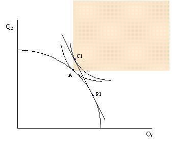t is possible to redistribute income to assure that everyone is absolutely better with trade than they were in autarky.

In other words, is it possible for the winners from free trade to compensate the losers in such a way that everyone is left better-off than they were in autarky?

The answer to this is yes in most circumstances. The primary reason is that the move to free trade improves production and consumption efficiency which can make it possible for the country to consume more of both goods with trade compared to autarky.

Consider the adjoining diagram. Point A on the PPF represents the autarky production and consumption point for this economy. The shaded region represents the set of consumption points which provide at least as much of one good and more of the other relative to the autarky equilibrium. Suppose in free trade production moves to P1 and consumption moves to C1. Since C1 lies within the shaded region , the country consumes more clothing and more steel in the aggregate than they had consumed in autarky. However, in moving from autarky to free trade some factors have experienced increase in income while others have suffered losses. This means that some individuals consume less of both goods in free trade while others consume more of both goods.

However, since there is more of both goods in the aggregate it is conceivable that government intervention which takes some of the extra goods away from the winners could sufficiently compensate the losers and leave everyone better-off in trade.

The possibility of an effective redistribution depends in some circumstances on the way in which the redistribution is implemented. For example, taxes and subsidies could redistribute income from winners to losers but would simultaneously affect the domestic prices of the goods which would affect consumption decisions etc., etc.. With the secondary effects of taxes and subsidies it becomes uncertain whether a redistribution policy would work. For this reason economists will often talk about making a lump sum redistribution or transfer. Lump sum transfers are analogous to the transfers from rich to poor made by the infamous character, Robin Hood. Essentially goods must be stolen away from the winners, after they have made their consumption choices, and given to the losers, also after they have made their consumption choices. Furthermore, the winners and losers must not know or expect that a redistribution will be made, lest that knowledge affect their consumption choices. Thus, a lump-sum redistribution is exactly what Robin Hood achieves. He steals from the wealthy, after they've purchased their goods, and gives to the poor, who were not expecting such a gift.

Compensation may not always be as straightforward as shown in the above example, however. Another possible outcome in a free trade equilibrium is for more of one good to be consumed but less of another relative to autarky. In other words the free trade consumption point may occur at a point like C1 in the adjoining figure. In this case it would not be possible to compensate everyone with as much steel as they had in autarky since the economy is consuming less steel in the free trade equilibrium. However, even in this case it is potentially possible to arrange a redistribution scheme. The reason is that the economy could potentially choose a consumption point along the pink line segment, as at point C2. Since the pink segment lies in the range in which more of both goods are available, compensation to make everyone better-off with trade remains a possibility.

Thus it is always potentially possible to find a free trade consumption point and an appropriate lump-sum compensation scheme such that everyone is at least as well-off with trade as they had been in autarky.

Factor-Price Equalization

The fourth major theorem that arises out of the Heckscher-Ohlin model is called the factor-price equalization theorem. Simply stated the theorem says that when the prices of the output goods are equalized between countries, as countries move to free trade, then the prices of the factors (capital and labor) will also be equalized between countries.

This implies that free trade will equalize the wages of workers and the rentals earned on capital throughout the world.

The theorem derives from the assumptions of the model, the most critical of which is the assumption that the two countries share the same production technology and that markets are perfectly competitive.

In a perfectly competitive market the return to factors of production depends upon the value of its marginal productivity. Marginal productivity of a factor, like labor, in turn depends upon the amount of labor being used as well as the amount of capital. As the amount of labor rises in an industry, labor's marginal productivity falls. As the amount of capital rises, labor's marginal productivity rises. Finally the value of productivity depends upon the output price commanded by the good in the market.

In autarky, the two countries face different prices for the output goods. Different prices alone, because it affects the value of marginal productivity is sufficient to cause a deviation in wages and rentals between countries. However, in addition, in a variable proportions model, different wage and rentals also affects the capital-labor ratios in each industry which in turn affects the marginal products. All of this means that for various reasons the wage and rental rates will differ between countries in autarky.

Once free trade is allowed in outputs, output prices will become equal in the two countries. Since the two countries share the same marginal productivity relationships it follows that only one set of wage and rental rates can satisfy these relationships for a given set of output prices. Thus free trade will equalize goods prices and wage and rental rates.

Since the two countries face the same wage and rental rates they will also produce each good using the same capital-labor ratio. However, because the countries continue to have different quantities of factor endowments, they will produce different quantities of the two goods.

Jeopardy Answers - Chapter 60

DIRECTIONS: As in the popular TV game show, you are given an answer to a question and you must respond with the question. For example, if the answer is, "a tax on imports", then the correct question is, "What is a tariff?"

1. nationality of the two economists, Eli Heckscher and Bertil Ohlin.

2. term used to describe Argentina if Argentina has more land per unit of capital than Brazil.

3. term used to describe aluminum production when aluminum production requires more energy per unit of capital than steel production.

4. general term used to describe the amount of a factor needed to produce one unit of a good.

5. the two key terms used in the Heckscher-Ohlin model; one to compare industries, the other to compare countries.

6. term used to describe when the capital-labor ratio in an industry varies with changes in market wages and rents.

7. term describing the ratio of the unit-capital requirement and the unit-labor requirement in production of a good.

8. the assumption in the Heckscher-Ohlin model about unemployment of capital and labor.

9. interpretation given for the slope of the production possibility frontier.

10. the H-O model theorem that would be applied to identify the effects of a tariff on the prices of goods and factors.

Problem Set 60-1

1. Suppose it requires 10 units of labor and 5 units of land to produce a ton of steel while it requires 2 units of labor and 4 units of land to produce a ton of wheat. Suppose the price of steel is $300/ton and the price of wheat is $100/ton.

A. Graph the lines along which the price and production cost are equal for steel and wheat.

B. What is the equilibrium wage rate and rental rate on land?

C. Suppose the price of steel rises to $350/ton. Graph the effect of this change on a new graph and find the new equilibrium factor prices.

D. Calculate the percentage changes of each output and factor price?

E. Construct the appropriate magnification effect relationship for prices for this example.

2. Imagine a two good H-O economy which imports automobiles and exports wheat. Suppose the production of these two goods use only capital and labor. If the government raises a tariff on the import of automobiles it will raise the domestic price of autos. Suppose the price of wheat remains constant.

A. Apply the magnification effect on prices to explain who in the economy will gain and who will lose because of the tariff? Be sure to state any additional assumptions needed to answer the question.

B. Are the effects described in part A short-run effects or long-run effects? Briefly explain why.

Problem Set 60-2

1. Suppose two countries, Malaysia and Thailand, can be described by a variable proportions Heckscher-Ohlin model. Assume they each produce rice and palm oil using labor and capital as inputs. Suppose Malaysia is capital-abundant with respect to Thailand while rice production is labor-intensive. Suppose the two countries move from autarky to free trade with each other. In the boxes below indicate the effect of free trade on the variables listed in the first column in both Malaysia and Thailand. You do not need to show your work. Use the following notation:

+    the variable increases -    the variable decreases 0    the variable does not change A    the variable change is ambiguous (i.e. it may rise, it may fall)

	in Malaysia	in Thailand
the price ratio Ppo/Pr
output of palm oil
output of rice
exports of palm oil
imports of rice
real wage in terms of palm oil
real wage in terms of rice
real rental rate in terms of palm oil
real rental rate in terms of rice
capital-labor ratio in palm oil production
capital-labor ratio in rice production

Problem Set 60-3

1. At the WTO Ministerial meetings in Seattle in 1999, opponents of the WTO argued that freer trade causes harm to many people in the country. Supporters of the WTO, however, argued that freer trade generates benefits for many people in the country. As our trade models suggest both sides are probably right. Show why this result is suggested in a Heckscher-Ohlin model by evaluating the redistributive effects of the following types of trade policies. Assume there are two goods, clothing and steel, produced with two factors, labor and capital. Suppose the country is capital-abundant and steel production is capital-intensive. Write down the magnification effect for prices when the country implements each of the following policies. Also specify who wins and who loses as a result of the policy. (Let P_S and P_C be the price of steel and clothing; let w and r be the wage rate and rental rates). [Hint: If a policy affects an import price, for example, assume the export good price remains unchanged]

	Magnification Effect	Winners	Losers
A. an import tariff
B. an export tax
C. an export subsidy

THE Heckscher-Ohlin theory states that each country exports the commodity which uses its abundant factor intensively. The HO theory was generally accepted on the basis of casual empiricism. Moreover, there wasn't any technique to test the HO theory until the input-output analysis was invented.

          What: The first serious attempt to test the theory was made by Professor Wassily W. Leontief in 1954.

          Result: Leontief reached a paradoxical conclusion that the US—the most capital abundant country in the world by any criterion—exported labor-intensive commodities and imported capital- intensive commodities. This result has come to be known as the Leontief Paradox. Leontief took the profession by surprise and stimulated an enormous amount of empirical and theoretical research on the subject.

          How: To perform the test, Leontief used the 1947 input-output table of the US economy (He received his Nobel prize for his contribution to input-output analysis later). He aggregated industries into 50 sectors, but only 38 industries produced commodities that enter the international markets, and the remaining 12 sectors were created for accounting identities and nontraded goods. He also aggregated factors into two categories, labor and capital. He then estimated the capital and labor requirements to produce:

          One million dollars' worth of typical exportable and importable in 1947.

	Capital Requirement	Labor Requirement
Exports	aKx = 2.550780	aLx = 182.313 man-years
Imports	aKm = 3.091339	aLm = 170.114 man-years

k_x = a_Kx/a_Lx = $14,300

k_m = a_Km/a_Lm = $18,200

     The US seems to have been endowed with more capital per worker than any other country in the world in 1947. Thus, the HO theory predicts that the US exports would have required more capital per worker than US imports. However, Leontief was surprised to discover that US imports were 30% more capital-intensive than US exports,

k_m = 1.30 k_x.

     At first, Leontief was criticized on statistical grounds. Swerling(1953) complained that 1947 was not a typical year: the postwar disorganization of production overseas was not corrected by that time.

Leontief's Second Test

     In 1956 Leontief repeated the test for US imports and exports which prevailed in 1951. In his second study, Leontief aggregated industries into 192 industries. He found that US imports were still more capital-intensive than US exports. US imports were 6% more capital-intensive

(k_m = 1.06 k_x).

Baldwin's Third Test

     More recently, Professor Robert Baldwin (1971) used the 1962 US trade data and found that US imports were 27% more capital-intensive than US exports. The paradox continued.

k_m = 1.27 k_x.

Trade Patterns of Other Countries

JAPAN

     Tatemoto and Ichimura(1959) studied Japan's trade pattern and discovered another paradox. Japan was a labor-abundant country, but exported capital-intensive goods and imported labor- intensive goods. Japan's overall trade patternwas inconsistent with HO.

Explanation: They said that Japan's place in the world was somewhere between advanced and LDCs.

25% of Japan's exports went to advanced industrial countries.

75% of exports went to LDCs.

For the US-Japan trade, the trade pattern was consistent with HO prediction.

Japan-LDC, consistent.

East Germany

     Stolperand Roskamp(1961) applied Leontief's method to the trade pattern of East Germany. East Germany's exports were capital-intensive. About 3/4 of EG's trade was with the communist bloc, and EG was capital abundant relative to its trading partners. Thus, the EG case was consistent with the HO theory.

CANADA

     Wahl (1961) studied Canada's trade pattern. Canadian exports were capital-intensive. Most of Canadian trade was with the US. The result was inconsistent with HO.

INDIA

     Bharawaj (1962) studied India's trade pattern. India's exports were labor-intensive. Consistent with HO theory.

          However, Indian trade with the US was not. Indian exports to the US were capital-intensive.

Explanations for the LP

Leontief: US was more efficient

     Leontief himself suggested an explanation for his own paradox. He argued that US workers may be more efficient than foreign workers. Perhaps U.S. workers were three times as effective as foreign workers. Note that this increased effectiveness of the American workers was not due to a higher capital-labor ratio, because we assume that countries have identical technologies and hence identical capital- labor ratios.

          It means that the average American worker is three times as effective as he would be in the foreign country. Given the same K/L ratio, Leontief attributed the superior efficiency of American labor to superior economic organization and economic incentives in the U.S. However, Leontief found very few believers among economists.

          Kreinin (1965) conducted a survey of engineers and managers, and tried to test whether an average American worker is three times as effective as a foreign worker. A realistic difference in effectiveness between the representative workers in the U.S. and those in the foreign countries were about 20-25%. Obviously, this difference does not explain the Leontief Paradox.

          When comparing trade patterns of a market economy and a command economy, this explanation may be important. Modern technology is available to Russians, but production in the former Soviet Union is still inefficient due to lack of incentives.

          Evaluation: There might have been some difference in labor efficiency or productivity between the US and the rest of world in 1947. But this should have been relatively insiginficant. This was probably a bad theory.

          Remark: Trefler (1993) resurrects Leontief's theory and has proved that when quality indices of factors are incorated, US exported capital and imported labor services in 1947 (HOV Theorem). This still does not prove, however, that US exports had been more capital intensive than its imports that year.

 

 

Factor Intensity Reversal

     If a commodity is produced by a labor-intensive process in the labor-rich country and also by the capital-intensive process in the capital-rich country, then factor intensities are reversed in the production of that commodity.

          Example: agriculture is labor-intensive in India but capital-intensive in US.

• If the US imports agricultural products, then an LP occurs in the US, because a capital abundant country is importing a capital-intensive product.

• If the US exports agricultural products, then an LP occurs in India, because a labor-abundant country, India, is importing a labor-intensive good.

          In the presence of FIR, the HO theory cannot hold for both countries. That is, an LP always occurs in one of the countries. Thus, Jones (1956) and Robinson (1956) argued that FIR could have been responsible for the LP in the US.

          The question is whether FIR is common in the real world. Minhas (1963) investigated 24 industries for which comparable data were available for 19 countries. He found FIRs only in 5 countries.

          Leontief (1964) reviewed Minhas's book and pointed out that only 17 out of 210 possible reversals did occur for the relevant range of factor prices. Moroney (1967) concluded that FIR has much less empirical importance, albeit theoretically interesting.

          Remark: Moroney was probably correct when comparing trade patterns with similar countries, or among developed economies. Capital-labor ratios are likely to be similar among developed economies and their resource endowments might be in the same cone of diversification.

 

While there has not been much empirical evidence about the possibility of factor intensity reversals, FIR is real. It may be important when comparing trade patterns between developing and developed economies (e.g. China vs. US).

Natural Resources

     Leontiefmay have oversimplified the production functions and failed to recognize the endowments of natural resources. With three factors of production, the HO model does not predict much. This is because the notion of abundance and intensity must be redefined.

Possibilities: factor abundance and intensity

K/L > K*/L* and K/N < K*/N*

K₁/L₁ > K₂/K₂ and K₁/N₁ < K₂/N₂.

Jaroslav Vanek's Argument (1963):

          Suppose the US is poor in natural resources. Assume that the import-competing industry uses capital and natural resources in fixed proportions. Then apply the HO theory. The US imports natural resource-intensive products, but it appears that the US is importing capital- intensive goods.

          Empirical studies have shown that the natural resource content in typical US imports is greater than that in US exports. But it is difficult to believe that US is poor in natural resources. Vanek's explanation is not very convincing.

Factor Abundance

In a world of many factors (K, L, N, .... Z), factor abundance can be ranked:

K/K* > N/N*> ...> L/L*.

     In this case, we can say that the HC is (most) abundant in capital, and least abundant in labor.

Heckscher-Ohlin-Vanek Theorem A country exports its abundant factors through trade in goods.

Let  = Y/(Y + Y*) be the home country's share of world income. Then the HC is abundant in capital, if

K/(K + K*) > .

Of course, this definition can be extended to any other factors. According to this definition, it is possible for a country to be abundant in more than one factors. The HOV Theorem states that if trade is balanced a country exports all of its abundant factors through trade in goods.

Remark 1. If factor prices are equalized, the definition of factor abundance makes sense, since income is the sum of factor incomes.

Y = wL + rK + sN + ...

In a world of two factors, if factor prices are equalized (w = w* and r = r*)

K/K* > Y/Y* if and only if K/K* > L/L*.

Thus, one can say that the above is a more general definition of factor abundance.

2. Trade theory is supposed to predict the patterns of output trade. As the number of outputs increases, it becomes exceedingly difficult to predict the patterns of output trade. Thus, HOV was not even a result that economists were looking for.

3. Nevertheless, HOV theorem predicts the indirect trade of factors through output trade. If HOV prediction is not materialized in the real world, it is an indication that there is a serious distortion in the economy. In this sense, HOV Theorem does provide a guide to trade policy; a trade policy should not encourage exports of scarce resources and imports of abundant resources.