9482-17866-1-SM

Fibírová and Šoljaková, 2005; Sedláček, Suchánek and Špalek, 2012). According to Wagner (2009), the performance of an enterprise is a characteristic that describes the way in which an enterprise carries out a certain activity similar to the way in which this activity is performed. Neumaierová and Neumaier (2002); Frost (2005); Šulák and Vacík (2005) are among the authors who understand the performance as the enterprise’s ability to capitalize its investments embedded into business in the best way.

1 Literature Review

Generally, we can state that business performance measurement means the assessment of its ability to achieve goals in the optimal way. The most common method of assessing business performance is the method of fundamental and technical analysis, which evaluates the enterprise in economic terms based on a detailed study and analysis of financial statements (Fisher, 1992). According to many Slovak and foreign authors (Ittner et al., 2003; Dixon et al., 1990; Pavelková and Knápková, 2009; Synek et al., 2007; Petřík, 2009), financial indicators, which include capital structure indicators, are used as the most common tools to measure the performance of companies. These conventional indicators map the main activities of the company in the areas of profitability, ability to pay, and investment area in terms of value for investors.

According to the argument that the objective is not only to measure, but in particular to improve performance (Hammer, 2007), it must be noted that these conventional financial ratios have a low predictive value in analysing and evaluating the financial performance of the company, in terms of making tactical and strategic decisions in management. This is caused by the fact that these results are judged rather isolated. Conventional performance indicators do not answer the question why the overall results achieve such values or which areas of the company should be improved in order to meet strategic company objectives. It is therefore important to supplement conventional financial indicators with other more dynamic and more prospective indicators, which are adjusted to specific competitive conditions. It means to focus on monitoring and comparing of implementation results describing performance with the planned level of performance, monitoring the strategies direction during their implementation, identifying the accompanying problems of fundamental importance, and performing the necessary changes and adjustments (Dudoková, 2004). Development of modern indicators of performance evaluation is focused on the processing and designing of indicators most closely connected to the value of shares. These indicators should also allow for usage of the most of accounting information and data, to include calculation of risk, to take into account the range of related capital, and finally, they should allow performance evaluation and also the enterprises’ valuation (Mařík and Maříková, 2005). The performance assessment should be approached from different perspectives: when assessing it from the shareholder’s position, the evaluation is based on return of invested capital into the company while every shareholder is expecting profitability adequate to risk (Neumaierová and Neumaier, 2002).

20

Therefore, basic financial fields of evaluation and measurement of business performance according to Kislingerová et al. (2011) can be supplemented by more recent and modern indicators and methods, namely evaluation using modern methods with the application of market characteristics such as indicators EVA, INEVA MVA, RONA, WACC or indicators based on FCF, CVA and others. From these indicators the best tool for performance measurement is Economic Value Added, which includes the impact of capital structure through capital structure risk used for Cost of equity evaluation.

One of the fundamental problems of business performance is to determine the correct composition of the funds needed to finance business activity, characterized by the term financial structure (Růčková, 2008). Capital structure is a less comprehensive term and expresses only the structure of long-term capital. According to another definition, capital structure informs users about the type of capital, the period during which funds are fixed, and business stability. It provides information on whether an enterprise makes optimal use of this capital in terms of indebtedness and capital commitment (Sedláček, 2003). According to Jánošová (2008), the company's capital structure is quantified using a wide range of indicators. The most commonly used indicators are: Total debt to total assets, Equity ratio, Debt to equity ratio, Equity to debt ratio, Interest coverage (key performance indicator, driver of the risk of capital structure), Interest burden, Equity to fixed assets ratio, Financial leverage, Stability and other indicators. Debt ratios create a network with strong relations between them (Štefko and Gallo, 2015), which results in the synergic effect of the indicators’ impact on business performance. Development of debt ratios for performance evaluation should be focused on the processing and design of indicators which are most closely connected to the performance evaluation (Suhányiová and Suhányi, 2011).

The idea of proper capital structure has been dealt with by many financial management experts. Several theories (static and dynamic theories on capital structure) have been processed and many views on the issue of sources of financing business activities (Závarská, 2012) have been published. An intensive discussion on this issue started when the original work by Modigliani and Miller (1958) was published. Frequently discussed was the issue of capital structure in terms of ownership that would maximize the economic profit and business performance. In general, these capital theories can be divided into two basic groups. The first group consists of static theories, the second of dynamic theories of capital structure. Static theories deal with the issue of optimal indebtedness and strive to answers the question whether there is optimal indebtedness, how to define it, on the basis of which criteria and in terms of who (the owners, managers or creditors). This group involves classic theory, traditional approach (U curve theory), theory of Miller and Modigliani (MM model), and trade off model. On the contrary, representatives of dynamic theories argue that there is no uniform methodology for determining the optimal capital structure due to the specific conditions of each enterprise. Dynamic theories include the theory of hierarchical order and the signalling model.

21

When deciding on business capital structure it is also important to assess from what amount of economic profit it is advisable to start using debt in addition to equity. For this purpose, the analysis of the point of indifference of the capital structure is used. It determines when it is appropriate to finance business needs by debt and when by equity (Jánošová, 2008). The capital structure is influenced by several factors, for example business risk, corporate tax position, financial flexibility, managerial conservatism and aggression (Růčková, 2008). In addition to these factors, the decision on the composition of capital is also influenced by business capital costs, namely Cost of equity, Cost of debt, and Cost of capital. For the calculation of the Cost of equity, a number of methods are presented in the theory. In this paper we applied valuation of Cost of equity with the use of Capital Assets Pricing Model – CAPM (with the acceptance of external, market, systematic risks) and Build-up model (with the acceptance of internal, specific, unsystematic risks). Cost of capital was calculated as Weighted average cost of capital (WACC). These models use quantification of the different risks that enter the valuation of capital. Therefore, when deciding on the business optimal capital structure it is necessary to quantify the risks and analyse the impact of risks arising from the capital structure on the valuation of capital and business performance.

Financial theory definitely confirms a certain link between capital structure and performance. In general, debt is cheaper than equity. A business owner accepts higher risk than the creditors, since the return on an investment for the creditors takes priority over the return on capital invested by business owners. Therefore, business owners require higher appreciation of capital invested in the enterprise. Increasing the share of debt in the financial structure of an enterprise can positively affect the amount of economic profit. On the other hand, with a rise in indebtedness, the risk of bankruptcy grows (Kiseľákova and Šofranková, 2015). This risk is gradually projected into the expectation of creditors who start to demand an increase in return on their investment to offset the risk they incur. The aim of the business owner is therefore to optimize the capital structure, with the intention of reducing the Weighted average cost of capital (WACC).

Research problem:

Does the company's capital structure affect business performance? What is business performance at a different equity to debt ratio? What is the impact of capital structure on Cost of equity and business performance? How does the capital structure affect Cost of equity evaluation calculated by CAPM (Capital Assets Pricing Model) and Build-up model?

2 Methodology and Data

The company under investigation is an electrical engineering stock company, which produces terminal telecommunication equipment such as standard, over-standard and special phones, residential equipment, electrical installation material, and others. The company's range of products is mainly oriented to the electrical engineering industry, but a large part of the production is focused on the

22

automotive and construction industries. The company's data for the years 20102016 were used as part of the analysis. From the capital structure point of view, company is financed by equity, while it does not have long-term liabilities. The average value of the indicator Equity ratio is 78%.

The aim of the paper was to find out the impact of capital structure on business performance.

Methods: In this paper we calculated the performance applying Economic Value Added (EVA), which is the best known and most utilized modern indicator of performance measurement. This model is known from the 1980s. Authors of the EVA model are representatives of Stern Stewart & Co., American researchers Joel M. Stern and G. Bennett Stewart III. The main task of EVA model is the measurement of business economic profit. Extensive use of EVA model dates back to 1989. We used EVA Equity and EVA Entity model for performance calculation. Formula (1) indicates that the Economic Value Added is expressed in two ways.

where stands for Economic Value Added, is Return on Equity, is Equity, and represents Rate of Alternative Cost of equity.

One formula shows what is known as the Spread ( − ), which expresses the relative ⁄ (Neumaierová and Neumaier, 2016). The relative EVA is needed as input to the correlation matrix.

Formula for the calculation of EVA Entity is as follows:

where stands for Net Operating Profit after Tax, is Weighted Average Cost of Capital, and represents Paid Capital.

Weighted Average Cost of Capital (WACC) is expressed by the formula:

where stands for Cost of debt, d is income tax rate applicable for evaluated business, and D represents market value of debt invested in the business (interestbearing).

For the calculation of Cost of equity, we used CAPM with the acceptance of market, external and systematic risks. This model is not used in its original format as it was processed by J. Treynor (1961 and 1962), W. Sharpe (1964) and J. Lintner (1965). These authors published articles about the CAPM model, which were processed in articles and publications of H. Markowitz, who dealt with the portfolio theory and risk diversification. W. Sharpe, H. Markowitz and M. Miller shared the Nobel Prize

23

for the application of CAPM model (Horváthová and Mokrišová, 2014). In this paper CAPM inputs were derived from the modified formula of Damodaran (2001):

where stands for Risk-free rate of return of US T-bonds, is Equity Risk Premium of US market, represents coefficient of systematic risk, and is Country Risk Premium (Damodaran, 2001). When calculating Cost of equity applying this formula, academics (Mařík, Maříková 2005; Horváthová, Mokrišová, Suhányiová 2016) recommend using inputs from the US market.

In order to compare performance results and the influence of risks on performance, we applied Build-up model for Cost of equity calculation. This model accepts internal - financial risks and internal and external business risks. It is used for the calculation of Cost of equity in the case we cannot use CAPM – it is the case when business shares are not traded on the stock market and β coefficient cannot be estimated. Build-up model is an empirical method of estimating the expected return on equity. It is a typical German approach to equity valuation. Its aim is to use as much factors as possible, therefore, it is often called comprehensive Build-up model (Vochozka et al., 2012). This method is based on the most complete consideration of individual risk factors (Osčatka, 2004). Principle of Build-up model is based on the assumption that independent variables are fundamental factors. Risk of these factors is evaluated and incorporated into equity valuation (Neumaierová and Neumaier, 2002). Based on the determination of fundamental factors, there are several Build-up models. Recent empirical studies of Fama and French showed that capital market accepts two risks (Neumaierová and Neumaier, 2002): risk of smaller companies in the form of risk premium for lower stocks liquidity in the market and risk arising from the fact that market value of business does not exceed its book value. Interest rate calculated with the use of Build-up model includes: risk-free rate of return (usually return on government bonds) and premium for specific risks. Main difference of this method compared to CAPM is that Build-up model does not include β coefficient, which represents systematic risk. Based on the above-mentioned, this method can be expressed by the formula:

where () is Cost of equity, rf is risk-free rate of return, RP is risk premium, which consists of various factors. In its basic classification it is divided into business risk factors, for example factors of market risk, factors related to size of the business and other specific factors (Štefko and Krajňák, 2013) and financial risk factors, for example the risk of fluctuations in cash flow. Risk Premium according to Mařík et al. (2011) is calculated using the following formula:

24

where stands for Risk premium for business risk and is Risk premium for financial risk (Mařík et al., 2011).

Due to the data compatibility, we used indicator Spread (⁄) as a relative performance measure. We applied this indicator in the correlation matrix and Principal Component Analysis.

Performance of the company measured by EVA Equity and also indicator Spread achieved negative values in most of the analysed years (Table 1). Cost of equity, which entered their calculation, was quantified applying CAPM.

Table 1 Development of company's performance

Source: Authors' elaboration

We chose Total debt to total assets, Equity to debt ratio, Current liabilities to total assets, Equity to fixed assets ratio, Interest coverage, and Financial leverage as the capital structure indicators. These indicators are closely linked to business capital structure and we also used them as the inputs for correlation matrix. Values of selected indicators are presented in Table 2.

Table 2 Selected capital structure indicators

Note: TD represents total debt,

TA total assets, E equity, FA fixed assets and CL current liabilities.

Source: Authors' elaboration

As already mentioned, the capital structure indicators show that the company's average indebtedness is at the level of 22%. This indebtedness is caused by shortterm liabilities. Values of Interest coverage are high because the company has low interests. The business is overcapitalized, has high Financial leverage and high Equity to debt ratio. These values are favourable to ensure business stability. On the other hand, it should be noted that these values negatively affect business profitability, which is a fundamental factor of performance.

25

We used correlation matrix processed in Software Statistica (Table 3) to analyse relationships between capital structure indicators and relative performance indicator Spread. In the correlation matrix, the correlations with P values lower than significance level of 0.05 were highlighted. To interpret correlation coefficient, we used Cohen (1998) scale according to which the absolute value of correlation coefficient above 0.5 is interpreted as a strong correlation, a value from 0.3 to 0.5 as a moderate correlation, 0.1 to 0.3 as a weak correlation, and a correlation coefficient value below 0.1 as a trivial correlation.

Table 3 Correlation matrix

Note: TD represents total debt,

TA total assets, E equity, FA fixed assets and CL current liabilities.

Source: Processed by authors in STATISTICA

The matrix (Table 3) shows that there is a strong, indirectly proportional relationship between Equity to debt ratio and Total debt to total assets, and there is a strong, directly proportional relationship between Total debt to total assets and Financial leverage. Similarly, there is a strong directly proportional linear relationship between Current liabilities to total assets and Total debt to total assets. In the case of Interest coverage, we did not notice a significant relationship with the analysed indicators. Interest coverage does not create a pair with any indicator because the way of its calculation is considerably different from the other indicators analysed. Interest coverage can be considered a key performance indicator that does not correlate with any indicator within the given group. None of capital structure indicators correlate with the indicator Spread. Based on the above mentioned, it can be stated that there is no significant relationship between the selected debt ratios and performance.

As the multicollinearity among capital structure indicators was confirmed, we applied Principal Component Analysis (PCA) processed in Software Statistica. With

26

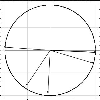
the use of this method, we verified the results obtained applying the correlation matrix. We applied the same capital structure indicators as in the correlation matrix and we identified two main components which involve 94% of the data variability. The first principal component evaluates Total debt to total assets, Equity to debt ratio, Financial leverage, and Current liabilities to total assets. The second principal component gives information about Interest coverage and Equity to fixed assets ratio (Figure 1).

Source: Processed by authors in STATISTICA

For the comparison of business performance in analysed years, we also constructed the plot of scores (Figure 2). It represents the coordinates of the analysed years in the new area defined by main components. Using the plot of scores, we can find out whether the performance in the analysed years is similar or whether they differ from each other.

Based on the plot of scores we can say that individual years differ in terms of performance. Quadrant A of the plot of scores (top left quadrant in Figure 2) houses years 2012 and 2013 in which the lower value of Total debt to total assets and Financial leverage negatively influenced business performance.

27

Figure 2 Plot of scores

Legend: Quadrant A – 2012, 2013; Quadrant B – 2010, 2011; Quadrant C – 2014;

Quadrant D – 2015, 2016

Source: Processed by authors in STATISTICA

Years 2010 and 2011 in which the higher value of Total debt to total assets and Financial leverage positively influenced business performance are located in quadrant B of the plot of scores (top right quadrant in Figure 2). In the year 2011 the analysed company also achieved a positive value of EVA indicator.

The lower value of Total debt to total assets and Financial leverage and the higher value of Equity to fixed assets ratio negatively influenced business performance in the year 2014 located in quadrant C of the plot of scores (bottom left quadrant in Figure 2). These results were distorted by the extreme value of Interest coverage.

In the years 2015 and 2016 located in quadrant D of the plot of scores (bottom right quadrant in Figure 2) the higher value of Total debt to total assets and Financial leverage positively influenced business performance but these results were distorted by the extreme values of Interest coverage too.

To confirm the impact of capital structure and cost of capital on performance, we used multiple linear regression model processed in software Gretl. Since the correlation matrix did not confirm significant relationships between capital structure indicators and indicator ⁄, we did not apply capital structure indicators as independent variables in regression models. Instead of them, we used equity, debt,

28