

The
total alignment time for different coarse threshold powers and
settling times, all using a raster coarse algorithm, are shown in
Figure 6.17. The total alignment time scales linearly with settling
time from 1000ms down to 300ms. However, experiments using settling
times <300ms consistently failed due to insufficient time for the
fiber to reach its new position. For a single settling time, we
observed that lower coarse threshold powers (50% vs 75%) produced
faster overall alignment results, but this improvement comes with
higher risk of getting trapped in side peaks during fine alignment.
Since the ribbed InP waveguide had insignificant side modes, this
trapping was not a problem. Overall, the total alignment time for a
single waveguide location was reduced from 34.2 seconds to 8.5
seconds by decreasing the settling time (from 1000ms to 300ms) and
coarse threshold level (from 75% to 50% peak). While the position and
sharpness of the target will influence the exact alignment times,
these trends should be universal.
1000ms,
1000ms, 500ms, 500ms, 300ms, 300ms,
75%
50% 75% 50% 75% 50%
Figure
6.17: Alignment times to an InP waveguide for different settling
times and coarse threshold power (% peak).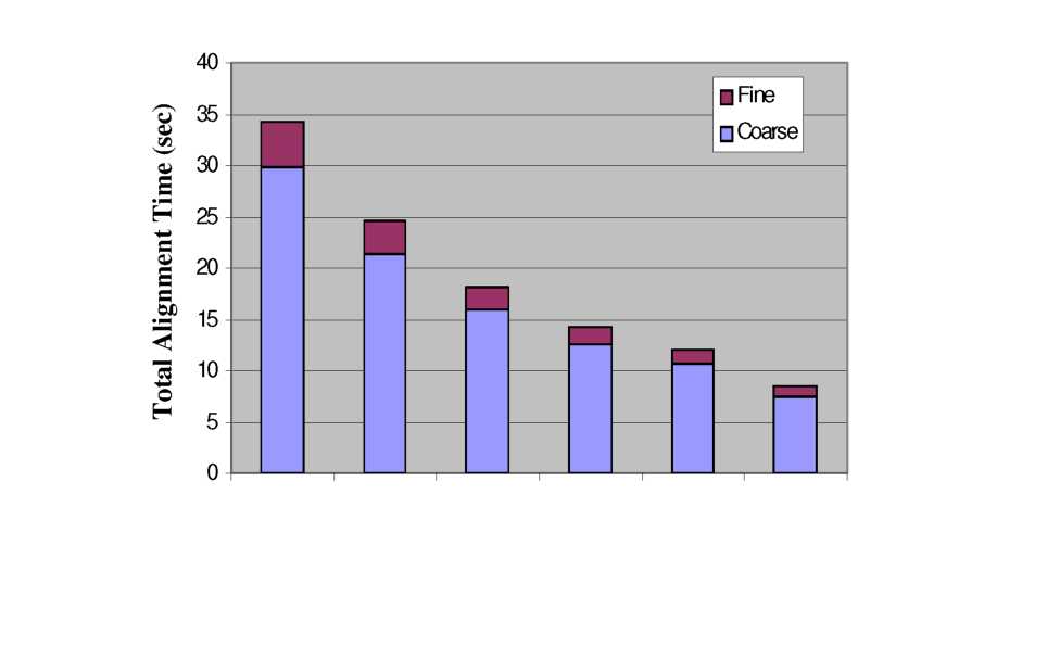
Settling Time, Coarse Threshold Power (%Peak)
It is obvious that for all cases in Figure 6.17, the total alignment time is dominated by achieving a coarse threshold power. Thus, some changes to the experimental conditions were implemented. First, we wanted to compare results when the raster coarse algorithm was replaced with the spiral coarse algorithm. And second, a 2p,m square InP waveguide (tighter optical confinement than ribbed waveguide) was used in conjunction with a final threshold of 95% peak coupled power to decrease the required alignment resolution to 1.6p,m (rather than the unimpressive 3.5p,m). Once again, the InP waveguide was fixed in a single location approximately ~20p,m vertically shifted from the gray-scale fiber aligner. The time required to achieve final alignment (<1.6p,m) was then recorded as it relates to coarse algorithm selection (raster vs spiral) and incremental actuator step size (AVoltage2 applied to comb-drives). The results are shown in Figure 6.18. Note that alignment results to a single target location were extremely repeatable (At<0.1sec).As expected for a quasi-centrally located target, the coarse alignment time dominates the total alignment time when a raster algorithm is used, especially for smaller AV2 (a finer scan mesh). Using the spiral algorithm dramatically decreased the coarse alignment time, but large AV2 increments caused the fiber to temporarily overshoot the target location. The fastest alignment times (routinely <10 seconds) were achieved using the spiral algorithm in conjunction with the smaller AV2.
Cleaved Fiber - Lensed Fiber (Resolution)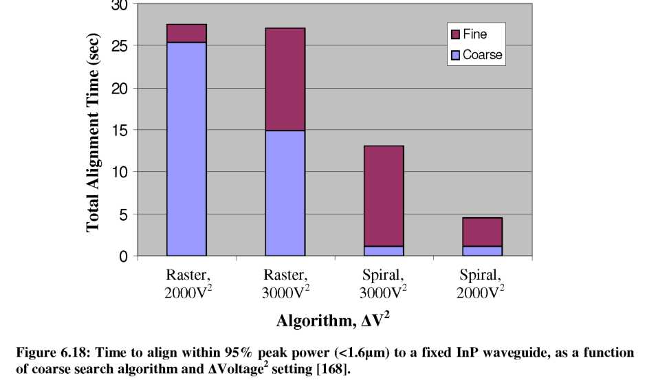
The previous experiments have established that high resolution alignment can be
obtained quickly to a few particular points in the gray-scale fiber aligner range. However, the achieved resolution (<1.6pm) in the InP waveguide experiments could have been an artifact of the particular waveguide locations tested. To fascilitate testing of many target locations, the InP waveguide was replaced with a lensed fiber on the electrostrictive XYZ stage as the new target. This setup enables quick reconfiguration of the target location (i.e. lensed fiber) to determine if high resolution can be achieved over the majority of the alignment area.
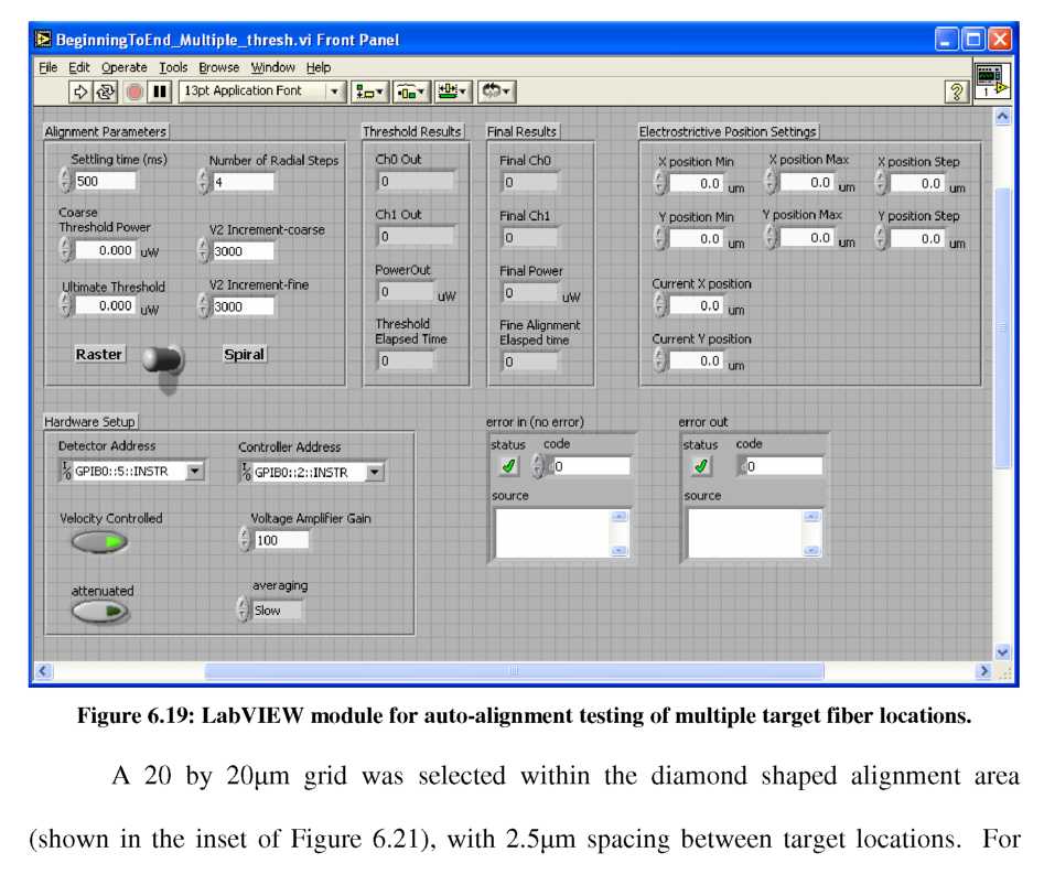
The custom LabVIEW module developed for executing the alignment tests at multiple target locations is shown in Figure 6.19. Universal hardware setup parameters are controlled in the bottom left section. The operator then selects either “raster” or “spiral” coarse search algorithm via a toggle switch, with the associated power threshold levels and AV2 increments. The position of the XYZ stage with lensed fiber is controlled using the “Electrostrictive Position Settings” on the right side. For each position of the XYZ stage and target fiber, the chosen alignment algorithm is executed and alignment results for both the coarse and fine steps are displayed and logged for analysis.
Estimated
Alignment Accuuacy (^m)
Figure
6.20: Estimated alignment accuracy histogram for 20 by 20^m area
using standard actuation.
Upon
further inspection, the problem with failed alignments was
identified to be between our actuator and the hill-climbing
algorithm. Typically, hill-climbing algorithms step towards a peak
and after passing a peak, turn around and scan again with a reduced
step size. (For intuition on the step sizes required for this level
of alignment, refer back to Section 6.2.3 where IUI=1000 created
3-4p,m of movement). However, small step sizes did not always cause
any appreciable movement, an effect we attribute to static friction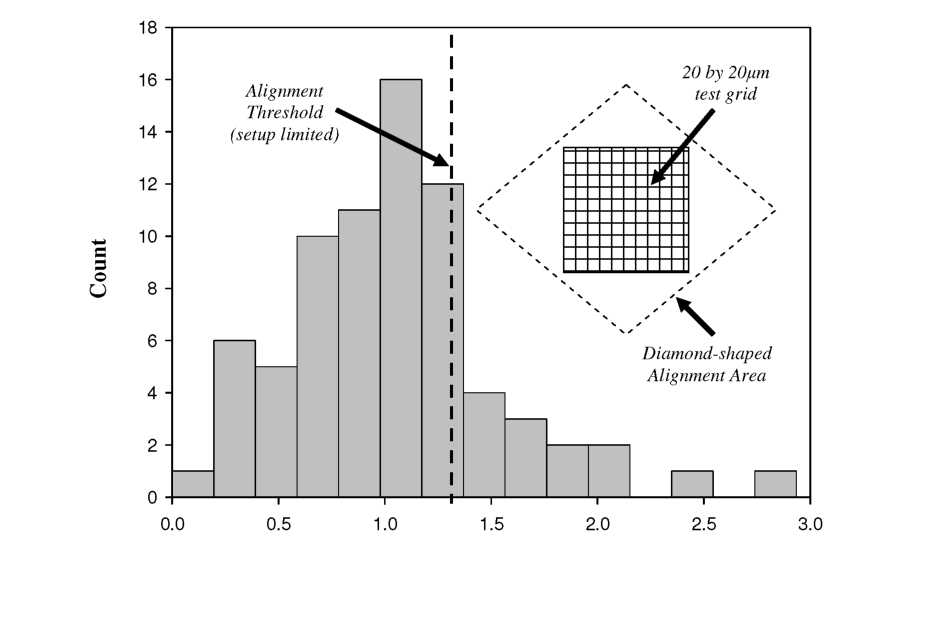
between the wedges and fiber. Thus, depending on target location, hysteresis, and friction conditions, decisions within the algorithm were often based simply on noise, causing the alignment to eventually fail.
We then altered the fiber actuation scheme to include a 100ms pulse of (0 V, 0 V) prior to the intended actuation voltage to “un-stick” and reset the fiber. While this method slows alignment slightly, it enables small AV2 steps to create real changes in the fiber location. Alignment tests were then performed over the same 20 by 20p,m area, but now using this ‘pulse’ method of actuation in the fine alignment step. As shown in the histogram of the estimated resolution in Figure 6.21, the 1.25p,m required threshold was achieved with 100% success across the entire area (all 81 measured points).