The primary drawback of the hill-climbing technique is the susceptibility to trapping in false peaks. This limitation can sometimes be addressed using a quasi­momentum term within a hill-climbing algorithm [171]. Alternative fine alignment algorithms have been developed that work better in the presence of side modes, such as the simplex method discussed in [175]. However, these algorithms can be quite complex, making it difficult to distinguish between algorithm complications and actuator performance. Since the targets used in this research operate with a single fundamental mode, and the coarse threshold is intended to avoid side modes, a hill-climbing algorithm is sufficient for this device characterization.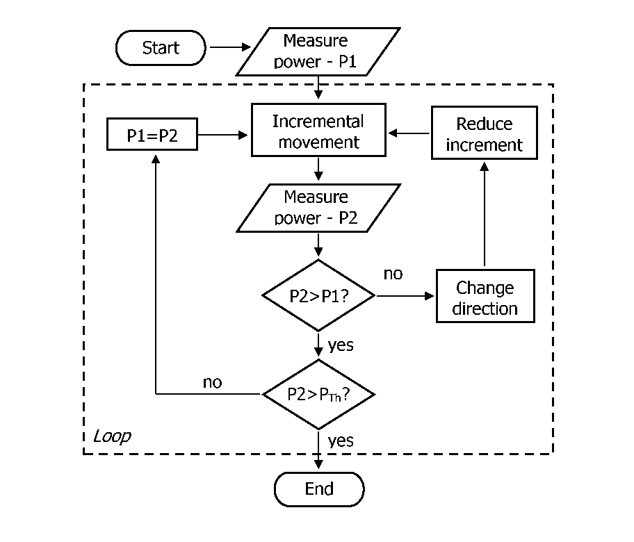

Figure 6.16: Simplified hill-climbing algorithm block diagram.

The most important parameters to be used during the hill-climbing algorithm are the step sizes and the ultimate fine threshold power. The initial step size determines how coarse a mesh the first 1-D search will be, and after each reversal of direction the step size is reduced (typically by */2). Large step sizes will climb the hill fast, but may over­shoot the optimum position and require many step size reductions to achieve the resolution required for final alignment. Small step sizes will take longer to climb a single hill, but should finalize alignment quickly once there. Use of small steps does make one more vulnerable to local false peaks caused by either secondary modes or artifacts of actuator motion (like sticking or hysteresis). Ideally, a compromise must be found between speed and reliability. A time-out function was also included to avoid infinite attempts to climb a hill that peaks outside of the possible area.

5. Automated Fiber Alignment Results

The experimental results presented in this section were performed entirely using the developed test setup described in Section 6.2. These tests were intended to specifically investigate the performance and limitations of the gray-scale fiber aligner using the implemented auto-alignment algorithms discussed in the previous section. Of specific interest are both the speed and resolution of the alignment process, each of which is focused on independently in the following two sections. Note that these tests make use of either lensed fibers or InP waveguides with approximately circular modes. While elliptical targets (like LEDs) may provide more coupling sensitivity along 1-axis, each power could correspond to multiple misalignment positions, significantly complicating evaluation of our device.

1. Cleaved Fiber - InP Waveguide (Speed)

The first auto-alignment tests using the gray-scale fiber aligner investigate the effect of algorithm parameters on speed of alignment within the constraints of the developed actuator and test setup. All experiments in this section utilized InP suspended waveguides (courtesy of fellow MSAL graduate student Jonathan McGee) [167] in an attempt to simulate in-package alignment to III-V photonic devices. It must be noted that due to the sensitive coupling between both facets of InP waveguides, alignment tests to InP waveguide were performed for a limited number of waveguide positions.

Initially, InP ribbed waveguides (2 by 2pm core with 400nm rib height) [167] were used as the alignment target, vertically misaligned by ~20pm with respect to the gray-scale fiber aligner. The waveguide location was somewhere towards the middle of the aligner’s range, but the precise location was left unknown to simulate ‘blind’ alignment. The final alignment threshold used for this first test was 92% peak, corresponding to ~3.5p,m misalignment due to the wide central mode emerging from the ribbed waveguide. While this resolution is far from the micron-level goal of this research, these tests serve to ensure that all alignment algorithms were implemented correctly.