

Figure
6.12: Force diagram during the “up” portion of a hysteresis
test, where the frictional forces oppose the net force acting on
the fiber from each alignment wedge.
It
should be possible to reduce this hysteresis effect by improving
the wedge morphology through a combination of design and/or
fabrication, although the observed roughness is already small
(1-2p,m) compared to the 125p,m fiber. Since the fundamental
principle of operation of this device relies upon two sliding
surfaces, it is not expected that hysteresis could be totally
eliminated in practice. As will be shown in later sections, fiber
alignment using closed-loop control has proven robust with the
current structures despite these small hysteresis effects.
Figure
6.13: Actuating both sloped wedges identically creates a vertical
up/down motion that exhibits definite hysteresis [168].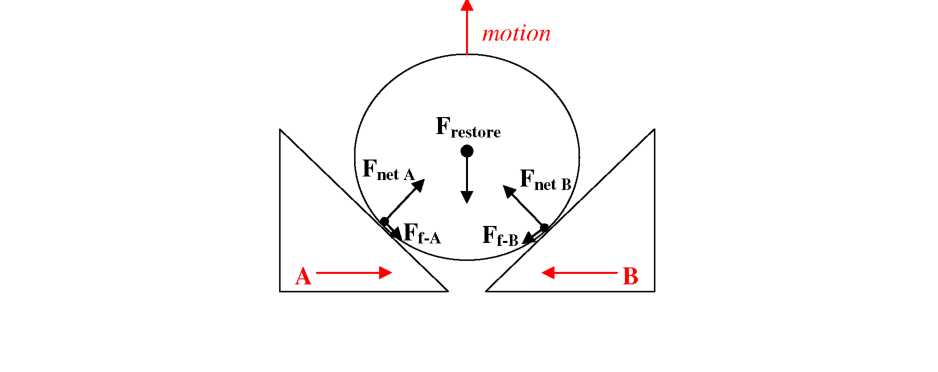 These
frictional forces between the wedges and optical fiber will oppose
the fiber motion on any actuation path, causing hysteresis. To test
the magnitude of this effect, a fiber was fixed with a vertical
offset compared to the gray-scale fiber aligner. During a sequence
of increasing then decreasing voltages, the gray-scale fiber aligner
tip passes through the point of peak coupling both on its way “Up”
and on its way back “Down.” The coupled power between fibers was
then measured as the gray-scale fiber aligner was fiber
motion, primarily caused by the morphology of the gray-scale wedges.
The main forces on the fiber during an “Up” cycle are shown in
Figure 6.12, where both wedges move towards each other to create
purely vertical motion. In the absence of friction, each wedge
transmits the electrostatic force of the comb-drive into a net
angled force on the fiber (Fnet
a
and Fnet
B).
These forces combine to produce a net force/movement “Up,” which
is balanced by a restoring spring force (Frestore)
that points back toward the original fiber location (“Down” in
this case). However, as the fiber slides “Up” each wedge, there
is a frictional force on each wedge face (F/_A
and Fj.b)
that will oppose the fiber’s upward motion.
These
frictional forces between the wedges and optical fiber will oppose
the fiber motion on any actuation path, causing hysteresis. To test
the magnitude of this effect, a fiber was fixed with a vertical
offset compared to the gray-scale fiber aligner. During a sequence
of increasing then decreasing voltages, the gray-scale fiber aligner
tip passes through the point of peak coupling both on its way “Up”
and on its way back “Down.” The coupled power between fibers was
then measured as the gray-scale fiber aligner was fiber
motion, primarily caused by the morphology of the gray-scale wedges.
The main forces on the fiber during an “Up” cycle are shown in
Figure 6.12, where both wedges move towards each other to create
purely vertical motion. In the absence of friction, each wedge
transmits the electrostatic force of the comb-drive into a net
angled force on the fiber (Fnet
a
and Fnet
B).
These forces combine to produce a net force/movement “Up,” which
is balanced by a restoring spring force (Frestore)
that points back toward the original fiber location (“Down” in
this case). However, as the fiber slides “Up” each wedge, there
is a frictional force on each wedge face (F/_A
and Fj.b)
that will oppose the fiber’s upward motion.
Voltage Squared (v2)
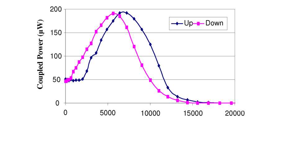 actuated
“Up” and “Down” over multiple cycles. As shown in Figure
6.13, there is definite hysteresis between the two actuation paths.
(While a single cycle is shown here, the hysteresis is quite
repeatable). Essentially, friction from the wedge surfaces increase
the force (i.e. V)
required to move the fiber “Up,” and then delays the fiber’s
return “Down” to a lower state. Using facet scans taken with the
calibrated electrostrictive stages, this ‘lag’ is estimated to
be equivalent to a shift of ~4p,m between the two coupling peaks.
actuated
“Up” and “Down” over multiple cycles. As shown in Figure
6.13, there is definite hysteresis between the two actuation paths.
(While a single cycle is shown here, the hysteresis is quite
repeatable). Essentially, friction from the wedge surfaces increase
the force (i.e. V)
required to move the fiber “Up,” and then delays the fiber’s
return “Down” to a lower state. Using facet scans taken with the
calibrated electrostrictive stages, this ‘lag’ is estimated to
be equivalent to a shift of ~4p,m between the two coupling peaks.
Auto-alignment Algorithms
The motivation for developing the gray-scale fiber aligner is rooted in automating the optical fiber alignment and packaging process. Thus, it is only prudent to demonstrate the capabilities of said actuator for auto-alignment of a fiber to various targets. Alignment algorithms can be considered a field unto itself and the development of entirely new algorithms is not the primary focus of this work. Rather, the following sub-sections will provide a brief overview of general alignment schemes, and focus instead on the adaptation of popular alignment schemes to the gray-scale fiber aligner. Of primary interest will be the impact and/or limitations imposed by the developed novel fiber actuation mechanism on the achievable alignment time and resolution.
Overview and Background
The majority of alignment algorithms developed in the literature utilize external
stages or fiber positioners capable of manipulating the fiber position in multiple axes [169-176]. Nearly all alignment sequences make use of multiple algorithms in order to minimize cycle time and improve reliability. Most begin with a coarse alignment step to achieve “first light” and meet some intermediate threshold power. This coarse threshold power is often designed high enough to avoid noise and secondary peaks. Once coarse alignment has been reached, a fine alignment step optimizes the alignment via a different algorithm.
The majority of alignment algorithm implementations use a “step-and-read” approach, where the fiber is moved incrementally and the coupled optical power is measured at the new fiber location. “If-then-else” types of logic are popular [174], however more complicated Hamiltonian [170] or fuzzy logic [171] approaches have potential advantages for simultaneously aligning many fibers with multiple degrees of freedom. Some algorithms also take advantage of a priori knowledge regarding the expected coupling profile shape (such as beam ellipticity) to reduce the overall alignment time [176].
The coarse and fine algorithms implemented in this work are adaptations of standard algorithms in order to characterize the performance of the gray-scale fiber aligner. To this end, our testing uses targets with symmetric coupling profiles, allowing us to infer alignment accuracy regardless of the direction of misalignment. After characterizing the performance of the gray-scale fiber aligner and demonstrating its flexibility, it would be possible to implement more complex alignment algorithms, but is considered beyond the scope of this work.
The coarse and fine alignment experiments discussed in the rest of this chapter will follow the same general sequence: (1) the longitudinal separation between the target and gray-scale fiber aligner is set manually under a microscope. (2) Electrostrictive XYZ stages are controlled via LabVIEW to create a facet scan of the target in order to correlate the coupled power to positional misalignment. (3) The target is intentionally misaligned with regards to the gray-scale fiber aligner. (4) A LabVIEW program, utilizing coarse and/or fine algorithms, optimizes alignment by modifying voltages supplied to gray-scale fiber aligner while monitoring the coupled optical power. (5) Upon satisfying all relevant thresholds, or giving up due to some failure, pertinent data is logged electronically. (6) Finally, the facet is re-scanned via the electrostrictive XYZ stages to verify that negligible drift occurred during the test(s).
Coarse Algorithms
We have implemented two separate coarse alignment scans using the gray-scale
fiber aligner to show its versatility and evaluate achievable speed and accuracy. It will be shown that the fundamental choice and settings of each algorithm has a significant effect on the speed with which the threshold is reached. For these coarse algorithm tests, cleaved fiber-cleaved fiber coupling was used for simplicity and ease of re-configuration. Coarse threshold powers of 50-75% peak power were typically used to simulate avoidance of side modes, but the observed coupling profile remains a single Gaussian- shaped peak as shown earlier.
The simplest coarse alignment routine is that of a raster scan. The voltage on the 1st actuator is held fixed, while the voltage on the 2nd actuator is swept through its range. The voltage on the 1st actuator is then incremented, and the sweep repeated on the 2nd actuator. The primary variable to control during a raster algorithm is the step size between successive fiber locations (AV because we are using comb-drives). Using a raster scan coarse algorithm, Figure 6.14 shows the time required to achieve a coarse alignment threshold of 75% peak coupling for different positions of the target fiber. The slope of the alignment wedges cause the time contour lines to be tilted with respect to the X-Y axes, a result of the sequential angled fiber trajectories caused by sweeping the 2nd actuator from one extreme to the other, as indicated in the figure. Note that times >36sec in Figure 6.14 indicate failure to achieve threshold, loosely illustrating the diamondshaped possible alignment area of this device.
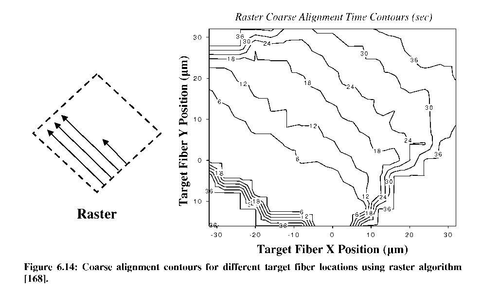
achieve coarse threshold scales by approximately the square of the step size ratio (AV old
22
 /
AV
new)
, essentially an area term. However, reducing the coarse alignment
time by using larger steps has the inherent risk of missing
important peaks altogether.
/
AV
new)
, essentially an area term. However, reducing the coarse alignment
time by using larger steps has the inherent risk of missing
important peaks altogether.
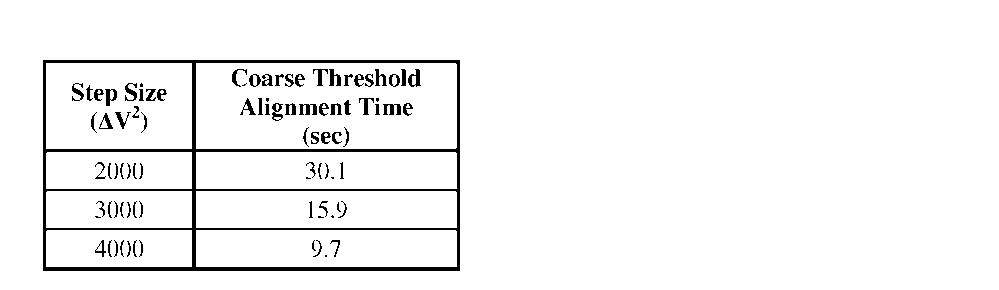
Table 6.5: Coarse alignment time to achieve 75% peak coupling as a function of step increment within raster algorithm for a single target location.
The primary drawback of a raster scan for packaging applications is that it begins searching for the peak in a presumably unlikely position (the very edge of the travel range at the bottom of the diamond alignment area). Ideally, an optoelectronic module design would have the target in the center of the alignment area such that shifts/errors in any direction could be corrected. However, even for perfect fabrication and assembly, a raster scan would still require 12-18 seconds to achieve coarse alignment to a centrally located target; meaning precise fabrication and assembly could require longer alignment times than in cases of poor assembly.
To address the paradox of perfect assembly requiring longer alignment times, a spiral search algorithm was also developed and implemented for the gray-scale fiber aligner to compare with the raster scan. Rather than beginning at the edge of fiber travel range, the spiral algorithm begins in the center of achievable motion, and spirals outward to progressively less-likely positions until the coarse alignment threshold is reached. Furthermore, a spiral scan is significantly more interesting from a device characterization standpoint since it requires coupled motion of both alignment wedges to create a spiral fiber trajectory (whereas the raster scan moves one alignment wedge at a time). The spiral trajectory used here was made of concentric circles of increasing radius. Both the radius of each ring and the angular spacing between successive fiber positions can be adjusted to tailor the speed and resolution of the fiber trajectory.
Figure
6.15 shows the measured coarse alignment time for the same target
positions as in the case of a raster scan. The time contours appear
in concentric circles, as expected from the desired fiber
trajectory. For locations near the center, we observed coarse
alignment times <6 seconds, confirming that the spiral algorithm
is more efficient when
the target is near the center, as likely in a packaging application.
It should be noted that the total time required to scan the entire
alignment area was kept approximately the same (>30sec) for both
raster and spiral algorithms to emulate a similar scan point density
in the X-Y plane.
Figure
6.15: Coarse alignment time contours for different target fiber
locations using a spiral algorithm [168].
Target
Fiber X Position (^m)
Spiral
Coarse Alignment Time Contours (sec)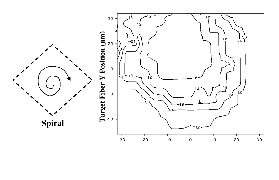
While only two basic coarse algorithms have been implemented so far, the spiral results clearly reinforce the previous claim that nearly arbitrary 2-axis motion of a fiber tip can be achieved through the coupled motion of sloped gray-scale wedges. Thus, any other 2-D coarse algorithm of interest could be implemented using the gray-scale fiber aligner.
Fine Algorithm
The ability to move a fiber tip in arbitrary patterns means that virtually any 2-D
search algorithm could be used for the fine alignment step. As mentioned previously,
Hamiltonian [170] and fuzzy logic [171] approaches tend to be most useful when aligning multiple fibers with many degrees of freedom, while the spot size method [176] requires 3 degrees of freedom and an optically elliptical target. The most popular algorithm for fine alignment is a “gradient search” or “hill-climbing algorithm” [174, 175] due to its simplicity of implementation.
A basic hill-climbing algorithm is shown in Figure 6.16. Coupled power measurements are taken at two successive fiber locations. If the coupled power increased, then the search continues in the same direction, “up” the hill. If the power change is negative, the algorithm assumes it is going “down” a hill, away from the optimum location. The search then turns around and reduces it’s step size (assuming it somehow jumped “past” the optimum peak because the step was too large). Since this process is 1-dimensional, the hill-climb loop for turning around is executed for each axis independently, usually switching between axes after every few changes in direction. This sequence continues until the ultimate threshold is reached (or the program gives up).