Figure 5.5: Calculated coupling as two co-axial single-mode fibers are separated longitudinally.

Thus, we can conclude that while the magnitude of fiber separation is important, active fiber positioning along the axis of transmission at the sub-micron level is unnecessary. Passive techniques for fiber placement along this axis can be utilized instead, meaning the gray-scale fiber aligner can restrict itself to 2-axis optimization of the more important axial and angular alignment components. Ultimately, for other devices or applications, the longitudinal fiber position may be more important than shown here, but positional requirements should still be more forgiving than along the other axes.

For the gray-scale fiber aligner, we will assume some constant separation value (Ztouii) between two fibers that are also offset both axially and angularly. The representative configuration is shown schematically in Figure 5.6. An input fiber is secured at one end to create a cantilever. The cantilever has an initial axial misalignment of Yo. The cantilever tip is then displaced (Ay) by the gray-scale fiber aligner in an attempt to maximize the coupled power. For the purposes of this analysis, we will assume that the misalignment in the x-direction (into the page) is negligible.

Figure 5.6: Alignment schematic for a bent fiber cantilever coupling to a fixed output fiber.

2 2Ay

The fiber cantilever length (L) and tip displacement (Ay) dictate the included angle (0) between the extended propagation axes of each fiber (see Appendix C):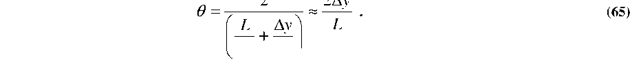

^Ay ^L J

For such separated fibers with an included angle (0), Joyce and DeLoach were able to show that the transmission (T) can be now be written as [158]:

The important aspect of Equations 66 and 67 is that the beam waists (w) must be evaluated at the appropriate (z) location corresponding to the intersection of the extended propagation axes. Thus, we can calculate the propagation distance for evaluation of w (Z_i and Z₂) based on the geometry of Figure 5.6:

Strictly speaking, the path traveled by the input beam will be the hypotenuse of the triangle created by Z_i and (Y₀-Ay). However, since the angles involved will be small for practical lengths and deflections (6<0.02 rad for L=5mm and Ay=50^m), Z_i is a reasonably good approximation of the path length.

Pure axial misalignment can be viewed as a special case of Equations 67 and 68, where the included angle becomes infinitesimally small angle (6=d/z as z^»). Thus, as z^», Equation 63 approaches w^2z/kw₀ and Equations 67 and 68 reduce to [158]:

These expressions are equivalent to those derived elsewhere for the case of pure axial misalignment of Gaussian modes [159].

As evident from the figure, the longitudinal loss caused by 30pm separation essentially causes a vertical shift across the entire range of tip displacements (0.31 dB). In contrast, the axial loss changes dramatically with tip deflection, where a 2pm

Figure 5.7: Various loss components for a single target fiber location @ У_й=20цт.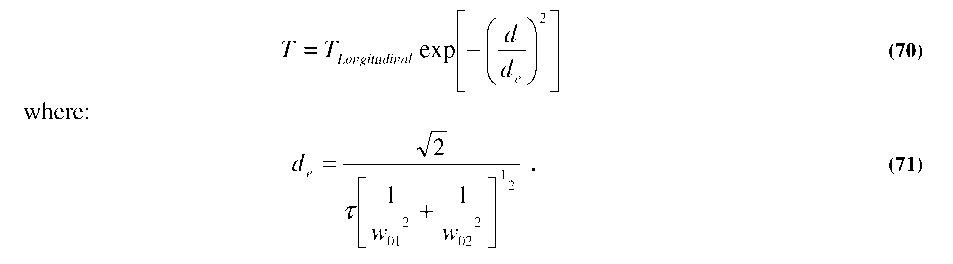

We will now use Equations 62-69 to simulate the transmitted power (T) as a function of fiber cantilever tip displacement and analyze the losses corresponding to each component. Shown in Figure 5.7 is the transmitted power for a cantilever (L=5mm) with various tip deflections. The target fiber location has been fixed at Y₀=20^m with longitudinal separation of Z=30^m. Also plotted in Figure 5.7 are lines indicating the loss that would be caused by each type of misalignment (longitudinal, axial, and angular) if they occurred independently of the other two. Strictly speaking, the three loss components are not entirely separable. However, for the geometries being considered, Figure 5.7 suggests that (to first order) they can be qualitatively viewed as components whose sum approximates the loss behavior near the coupling peak.

misalignment should cause >0.5 dB of loss. While the relative sensitivity to axial misalignment should be independent of target location, Figure 5.7 shows that the angular misalignment loss (0.03dB for Y₀=20p.m) increases with cantilever tip displacement (increasing 0). Since the gray-scale fiber aligner reduces the amount of axial loss by introducing a small angular loss, the location of the target fiber is extremely important as it dictates the angular loss penalty introduced by the device.

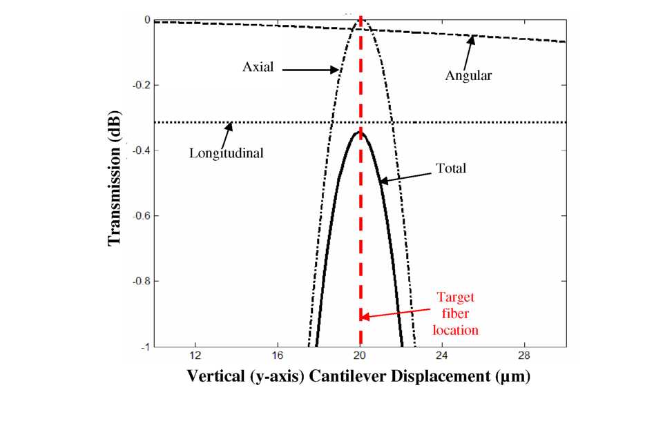
Looking more closely at the angular loss penalty, Figure 5.8 plots the maximum transmission for different fiber cantilever lengths and tip displacements (temporarily assuming no longitudinal separation). For long cantilevers (10mm), the angle created by bending the fiber tip 50pm is still rather small. However, for shorter cantilevers (5mm), the angle resulting from the same displacement is larger (see geometry analysis in Appendix C), leading to more optical loss. For comparison, the loss caused by 1pm pure axial misalignment is also shown.

We see that a 5mm cantilever with 45p,m tip displacement actually introduces greater angular loss than would be caused by 1p,m axial misalignment. This means that for cases of short fiber cantilevers and large deflections, the gray-scale fiber aligner may not provide a significant advantage over other alignment techniques. As a general rule, the angular loss introduced by the gray-scale fiber aligner should be small compared to the equivalent axial loss tolerance we are trying to obtain. Thus, Figure 5.8 illustrates that this device will have inherent limitations in actuation range when the length of the fiber cantilever is scaled down.

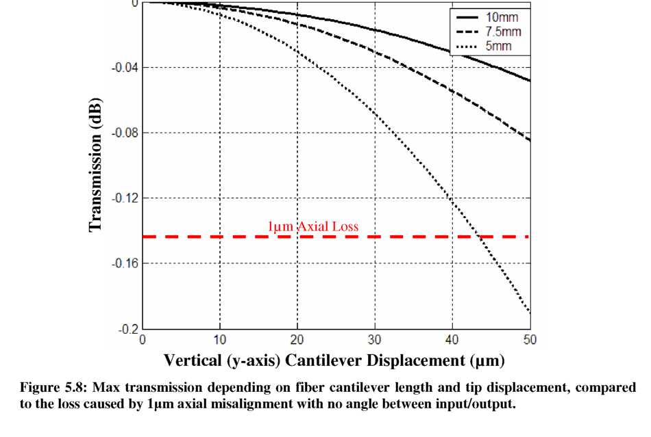
Another way interpret the introduction of angular misalignment is that the axial misalignment must be improved in order to compensate and maintain the same total transmitted power. This concept of angular/axial alignment tradeoffs has been derived analytically in multiple forms as an “alignment product” of angular and axial tolerance terms [158, 159]. Fiber splices requiring high axial resolution are insensitive to angular misalignment, while fiber splices requiring high angular resolution are less sensitive to axial misalignment. As the fiber tip is deflected by the gray-scale fiber aligner, many combinations of angular and axial losses occur. Thus, the power transmission curves for an L=5mm cantilever have been calculated numerically for different target fiber positions to investigate the tradeoff between tip deflection (angle) and required resolution (see Figure 5.9). The loss caused by a 1p,m axial misalignment is also plotted for reference.

As evident in Figure 5.9, target fibers located at large tip deflections have progressively lower peak transmission due to increased angular loss. Thus, axial alignment resolution must improve to <1p,m in order to surpass the equivalent of 1p,m axial misalignment with no tip deflection. Table 5.1 shows the maximum transmission

and axial resolution required to achieve coupling equivalent to a 1pm pure axial misalignment. We see that for a 5mm cantilever and a target fiber at Y₀=40^m, the axial resolution must improve from 1pm to 0.40pm to achieve power transmission equivalent to 1pm pure axial misalignment.

While a 1pm axial loss for cleaved fiber-fiber coupling has been used here for comparison purposes, the tolerances involved will be heavily device and application dependent (e.g. coupling to laser diodes with lensed vs. cleaved fibers has much different tolerances [162]). Most importantly, the preceding coupling analysis serves as a guideline

to estimate limitations of the proposed device. One must use similar analysis to determine what advantage the gray-scale fiber aligner can provide in a specific application.

In this research, to avoid significant angular loss, and for mechanical reasons discussed in the following section, fiber cantilevers with L>i0mm were used. For the lengths and deflections considered here, the radius of curvature for bent fibers is >1m, making bending losses inside the optical fiber negligible.

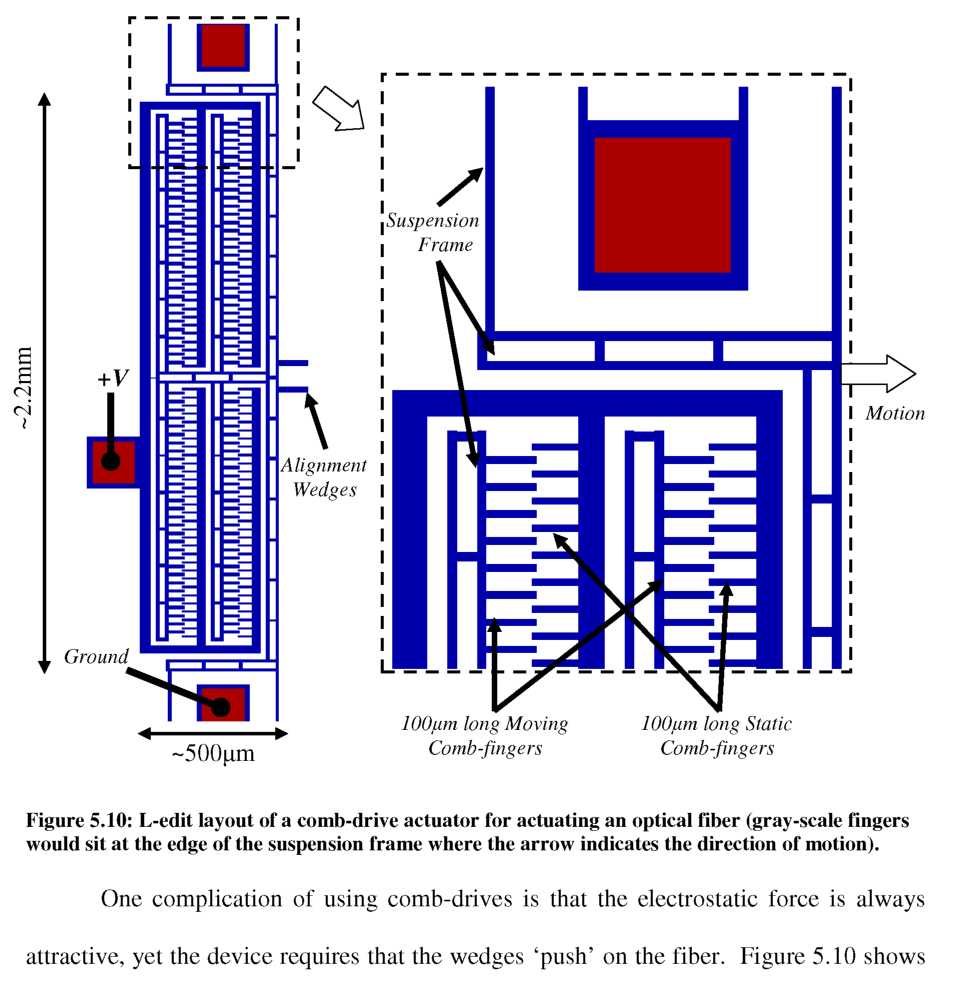
2. Design

The principle of operation of an out-of-plane actuator based on opposing sloped alignment wedges was shown previously in Figure 5.1. Translating the alignment wedges alters the location of a cylindrical optical fiber resting within a dynamic v-groove. Since initial embodiments in packaging applications will require only a single use, it is not required that the actuator be either low-voltage or low-power, allowing a large amount of flexibility in actuator design. Planar electrostatic MEMS comb-drives will initially serve as the actuation mechanism for translating the sloped alignment wedges. This enables the use of the same process flow to fabricate both comb-drives and sloped alignment wedges simultaneously. Future devices could integrate variable-height comb-drives for improved displacement resolution, but such improvements lie beyond the initial goals of this thesis. For feasibility in packaging applications, the gray-scale fiber aligner should be capable of compensating for accumulated packaging and assembly errors to the order of 10p,m initial misalignment [152]. The following sections discuss in more detail the design of the actuation mechanism and the design of the opposing sloped alignment wedges.

1. In-Plane Actuators (Comb-drives)

Design of the in-plane electrostatic MEMS actuator will largely focus on

achieving the desired fiber deflection magnitude. As shown previously in Figure 5.3, the anchor point for the optical fiber provides approximate passive alignment of the optical fiber, similar to a passive v-groove, such that the fiber’s free end rests between the sloped alignment wedges. The location of this anchor point determines the length, and therefore spring constant, of the cylindrical optical fiber cantilever, according to [163]:

3nEr^A

^k fiber = 4i 3 ^⁷²⁾

where E is Young’s Modulus of the fiber (~70GPa), r is the radius of the fiber (typically r=62.5jum), and l is the length of the fiber cantilever. As an example, a 10mm cantilever results in kfi_ber= 2.5 N/m. To first order, this spring constant can be modeled as part of the spring constant of the in-plane MEMS actuator suspension.

To achieve a desired range of motion, the actuation mechanism and fiber cantilever length must be considered jointly. Electrostatic comb-drive actuators have well-characterized force behavior, simplifying both design and control. The force generated by a comb-drive was presented earlier in Chapter 3 (Equation 29), and is repeated here:

£ h

F = N -°-V² (73)

d

where N is the number of comb-fingers, s₀ is the permittivity of free space, - is the comb- finger height, d is the gap between fingers, and V is the applied voltage. Making some basic assumptions (N=100, -=100p.m, d=10^m, V=100V), we can estimate a generated force of 89pN. If this force were applied directly to the fiber cantilever discussed above, the deflection would be >35pm (F=kx). However, one must also consider two additional factors for this device: first, the sloped wedges push the fiber at an angle, causing the fiber deflection magnitude to be slightly smaller than the comb-drive deflection (assuming 45° wedges). Second, part of the generated comb-drive force is used to bend the comb-drive suspension, reducing the force delivered to the fiber. However, it is still reasonable to expect fiber actuation on the order of 10’s of micrometers using comb-drive voltages of 100-150V on fiber cantilevers in the range of 10-12mm long. The use of comb-drive actuators also provides interesting possibilities for integrating the gray-scale comb-fingers discussed in Chapter 3 for improved positioning resolution of the fiber.

the novel approach taken in this research to create a “repulsive electrostatic comb-drive”. Starting from a single electrode, the static comb-fingers were arranged on arms that reached around and point back towards the aluminum (Al) contact pad. The suspended comb-fingers meanwhile are attached to a stiff suspension frame that extends between the static electrode arms. Upon applying a voltage to the Al contact pad, the suspended structures get pulled to the right by the wrapped-around comb-fingers. Thus, a pushing motion has been created from the perspective of the electrode. One drawback of this design is its size. Wrapping the suspension frame inherently takes extra space, and a device with 100 comb-fingers per side requires significant real-estate on the wafer. The area required for one side of the actuator shown in Figure 5.10 is ~1.1mm . Given the size of the suspensions (1mm long each) and length of the cantilever (~10-12mm), an entire device is in the range of ~7 mm.

For devices investigating the design, fabrication, operation, and control of this new type of actuator, the relatively large overall footprint is acceptable. However, for packaging applications, it is imperative that these systems be reduced in size, particularly for packaging of fiber arrays with a small pitch (250-500pm). Two primary approaches for developing such systems will be discussed in Chapter 7 as extensions of this work:

1. the use of reduced cladding fiber (r=40pm) for shorter/more flexible cantilevers, and

2. integration of higher force actuators that have potentially smaller footprints (such as thermal [45]).

The rest position of a fiber tip between sloped alignment wedges can be calculated using geometry (see Appendix D). We will always assume that the restoring force of the bent fiber cantilever causes it to rest at the bottom of the dynamic v-groove.