

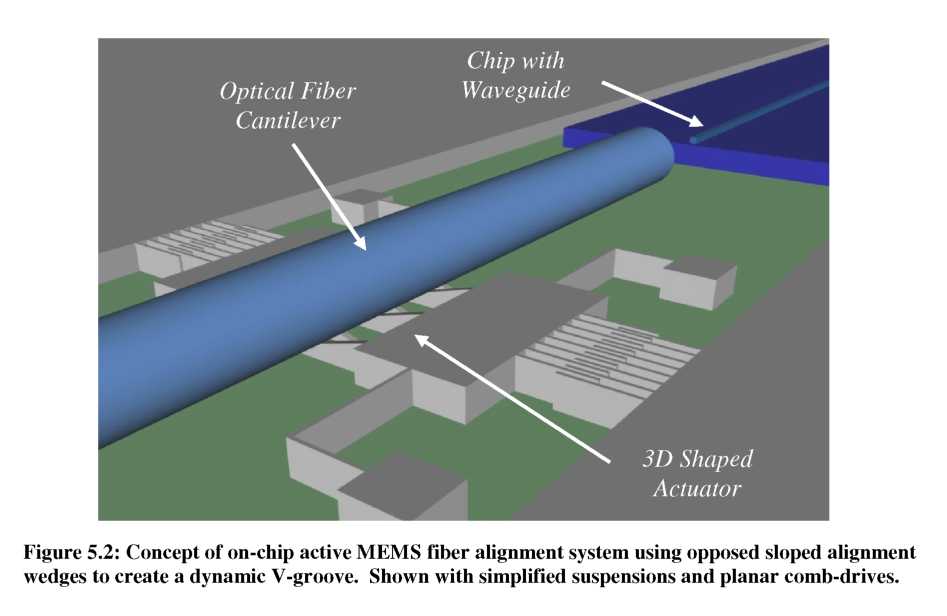
Device Concept
Contrary to traditional fixed v-groove designs obtained by wet chemical etching [78-83, 149], the fiber alignment mechanism developed in this research creates a dynamic v-groove using opposing sloped, silicon wedge structures to hold the optical fiber in a particular alignment location. The basic alignment mechanism is illustrated in Figure 5.1. In Figure 5.1(a), the system is “at rest” with the fiber lying at the bottom of the dynamic v-groove. However, in Figure 5.1(b), after an in-plane displacement of one silicon alignment wedge, the bottom of the dynamic v-groove has been translated in both the in-plane and out-of-plane directions, altering the alignment of the optical axis. Thus, through coupled in-plane motion of opposing wedge structures, alignment of an optical fiber in the X-Y plane can be achieved.

Figure
5.3: Top view schematic of the 2-axis optical fiber actuator [157].
The opposing actuators are aligned with a static v-groove trench to
provide approximate passive alignment.
Fiber
Coupling Loss Analysis
The
goal of the gray-scale 2-axis fiber aligner is to eliminate axial
misalignment by bending the fiber to an appropriate position.
However, bending the fiber inherently introduces some loss as well.
Thus, three primary sources of optical loss, shown in Figure 5.4,
should be considered and analyzed: longitudinal (along the axis of
light propagation), axial (perpendicular to light propagation), and
angular. The coupling analysis in this section is based on the
Gaussian coupling model presented by Joyce
and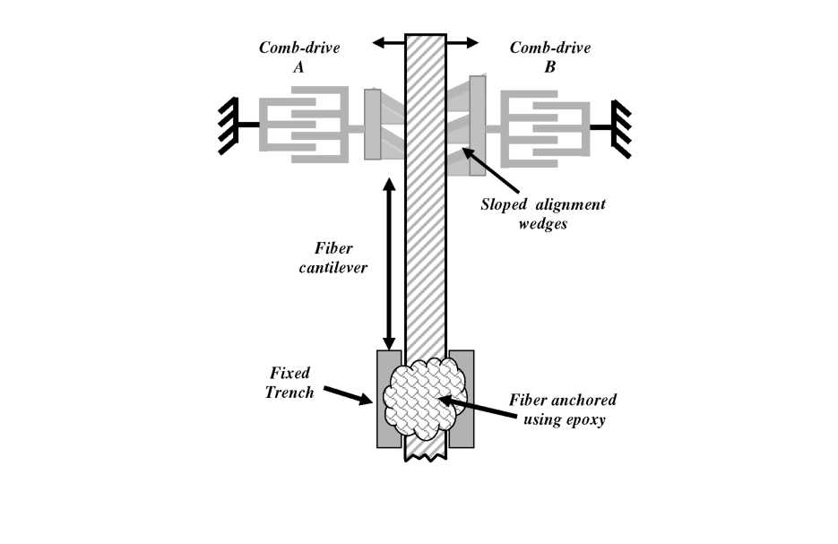
DeLoach in 1984 [158]; however adaptations have been introduced to specifically model the behavior of the gray-scale fiber aligner. This approach requires beams to be represented by their nearest equivalent Gaussian mode, which while an approximation, provides useful insight to the coupling for a variety of optical and mechanical configurations of the gray-scale fiber aligner. The following analysis will assume fiber- fiber coupling, but can be applied to other source/sink combinations with approximately Gaussian modes. Similar treatment of Gaussian coupling can be found in [159, 160].
b)
Axial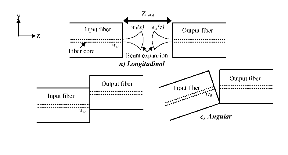
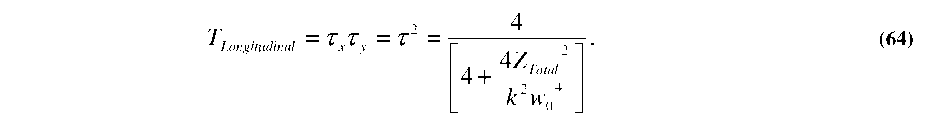
The simplest case to consider initially is that of purely longitudinal separation between two co-axial fibers, as shown in Figure 5.4(a). Since the optical mode is no longer confined upon entering the gap between the two fibers, the beam waist (W) will expand as it propagates in the z-direction according to:
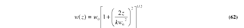
where k=2n/X and w0 is the original beam waist inside the fiber core. The term w is known as the half-width or beam waist, where the amplitude of the electric field drops to 1/e of the peak, or where the intensity drops to 1/e . For the simulations below, and most subsequent experiments in the following chapter, 8.2p,m core single mode optical fibers were used (Corning SMF-28e), with 2w=10.4jumf, and an operating wavelength of X = 1550 nm to match the preferred low loss window of optical fibers [161].
For elliptical mode profiles, the coupling efficiency (t) between co-axial fibers for either the x or у primary axes, can be calculated separately to be [158]:
 Material
data sheet (www.corning.com/photonicmaterials/pdf/pi1446.pdf,
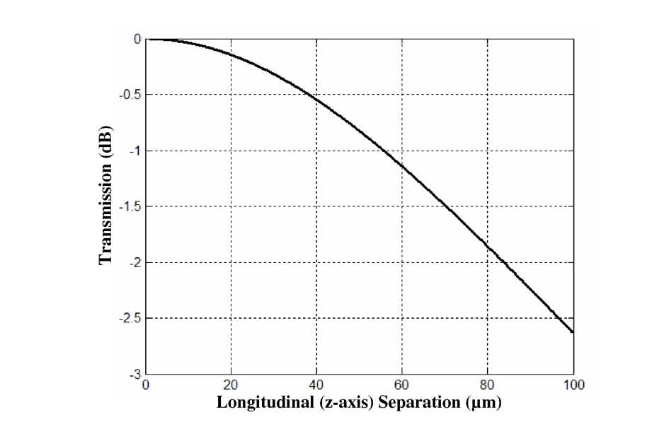
accessed 3/16/05).25pm
separation is <0.08dB. As will be shown shortly, this difference
in coupling is virtually negligible compared to the change in
coupling that would be caused by similar levels of axial
misalignment. Other studies have also shown the longitudinal axis to
be the least critical of the misalignment components considered here
[159, 160].
Material
data sheet (www.corning.com/photonicmaterials/pdf/pi1446.pdf,
accessed 3/16/05).25pm
separation is <0.08dB. As will be shown shortly, this difference
in coupling is virtually negligible compared to the change in
coupling that would be caused by similar levels of axial
misalignment. Other studies have also shown the longitudinal axis to
be the least critical of the misalignment components considered here
[159, 160].