4. Testing and Characterization

Static and dynamic characterization of all resonators was performed using an optical profiler (Veeco Wyko NT1100 with DMEMS option). As with the comb-drive testing in the previous chapter, the resonating mass and bulk substrate are kept electrically grounded to avoid pull-in forces normal to the substrate. The following sections will review the methods used to test each resonator, and to extract the resonant frequency (f) and electrostatic spring constant (kelec) as a function of tuning voltage.

1. Method

The Wyko NT1100 operates under the principle of white-light interferometry in both of it’s primary modes, static and dynamic. Pattern recognition software can be used in either mode to measure relative structure movements in both the horizontal and vertical planes.

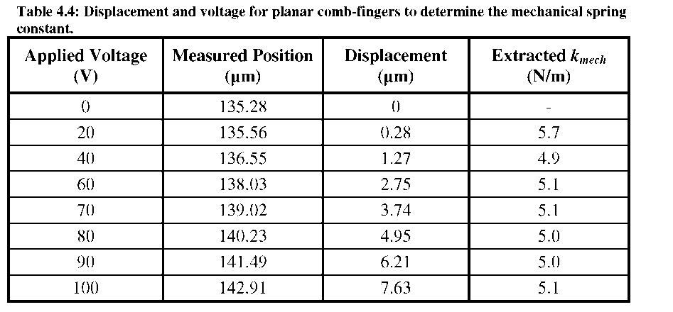
DC tests on the set of planar comb-fingers on each resonator were used to estimate the mechanical spring constant of the suspensions (k_mech). Analytical equations were used to calculate the force as a function of applied voltage (Equation 29 from Chapter 3), while the Wyko software was used to track the resonator position. The kmech is then back-calculated using F=k_mechx. Example displacement vs. voltage measurements are shown in Table 4.4, where the extracted kmech is relatively consistent.

Next, the dynamic measurement mode is used to determine the frequency response for different tuning voltages. In this mode, the Wyko uses an LED that is synchronized with the actuation signal to strobe the resonator at a particular phase of its periodic motion. A schematic of the periodic driving signal is shown in Figure 4.10, where the peak of the shifted sinusoid occurs at a phase of 90°.

To obtain the resonant frequency, we strobe the motion at a particular phase, while sweeping the actuation frequency. As the resonator passes through resonance, the drive signal and resonator motion will undergo a relative phase shift, according to the standard resonance equation [145]:

where S is the resonator displacement, F is the applied force (F=F₀sin(rnt)), Q is the quality factor, and is the resonant angular frequency. A brief inspection shows that as rn^0, Equation 55 reduces to Hooke’s Law (S=F/k_mech), while for the case of rn=rn_R (resonance) we find a -90° phase shift:

Considering this standard resonance behavior, depending on the choice of phase for the LED strobe, the measured resonator position vs. frequency will be quite different. Here we will discuss two primary examples: first, if a strobe phase of 90° is chosen, then for f<<f₀ the measured resonator position will be at its maximum deflection (during the

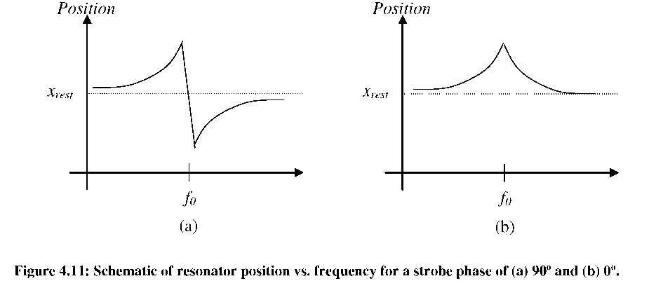
peak of the V_dri_ve signal). As the drive frequency approaches f₀, the resonant amplitude will gradually increase. However, at resonance, the 90° phase shift causes the mechanical vibration and LED strobe to be 90° out of phase. Thus, the resonator will now be strobed in the middle of its travel range, appearing as negligible movement even though the amplitude of vibration is maximized. As the frequency increases further to f>>f₀, another 90° phase shift causes the strobe and mechanical motion to be 180° out of phase, and the measured resonator deflection is at the maximum deflection in the opposite direction. This sequence is depicted in Figure 4.11(a), where the point that the resonator position crosses the rest position indicates the approximate point of resonance. Yet, the odd shape of such a plot makes it difficult to determine f₀ accurately with a limited number of data points.

Alternatively, a phase of 0° can be used when strobing the resonator. Initially, almost no motion is detected because the strobe occurs in the middle of any periodic motion. However, as the drive frequency approaches f₀, the 90° phase shift causes the maximum mechanical deflection to shift to the phase where it is being strobed. This method creates a plot of position vs. frequency similar to Figure 4.11(b). This second method is preferred for the purpose of determining resonant frequency because a peak curve fit can be used to extract the center frequency of the peak with only limited data points required. For the data discussed here, a 4-parameter (a,b,x₀,y₀) Lorentzian fit in SigmaPlot was used of the form:

The quality factor (Q) of a device is often estimated using Q=roo/Aro, where Дю is the full-width half max of the power spectrum, or 1/V2 of the amplitude. However, we must remember that the Wyko records the position of the resonator at a particular phase for each frequency, not the amplitude vs. frequency that is required to estimate the quality factor. Thus, the width of the Lorentzian fit to this data cannot be used to find Q. The Wyko is capable of generating amplitude vs. frequency plots, but requires a series of nested phase and frequency sweeps that is much more time consuming. However, referring back to Equation 56 for the case of m=m_R, we can divide the peak resonant amplitude by the displacement caused by a DC signal to obtain an approximate Q. For most resonators tested here, this method yielded Q’s of ~15 in air.

2. Weakening Resonator Tests

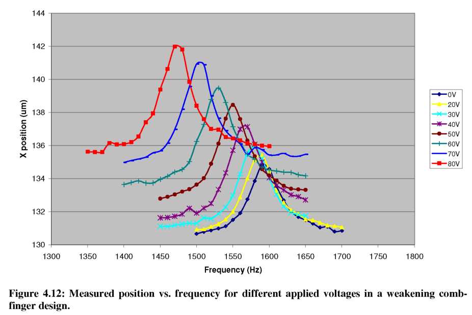
Tests of the weakening resonator design used an AC drive voltage of 30V on a

device with 10-20p,m gray levels and 10p,m wide suspension arms. The extracted k_mech from static tests was 4.7 N/m. Figure 4.12 shows the measured resonator position as a function of frequency for different applied DC tuning voltages (0-80 V). Notice that as the voltage is increased, the base of the peak shifts gradually in the +x direction by ~5p,m, as expected from the asymmetric resonator design and large DC tuning voltages. As the tuning voltage increases, the resonant peak shifts to lower frequency, consistent with a “weakening” of the mechanical spring in Equation 53. SigmaPlot curve fits show the resonant peak shifted from f₀= 1594.6 Hz at V_tune= 0V, to f_tuned= 1442.4 Hz at V_tune= 90V.

To compare these tuning results to our predictions, we start by taking our k_elec parameter from Figure 4.6 for the 20pm case at each appropriate finger engagement (accounting for the DC displacement caused by V_tune). Using V_tune and the number of comb-fingers (N=48), the expected k_elec is calculated for each voltage using Equation 50. This result was combined with the measured kmech in Equation 54 to yield a predicted resonant frequency as a function of tuning voltage. The measured and predicted resonant frequencies match well, as shown below in Figure 4.13.

3. 

   Stiffening Resonator Tests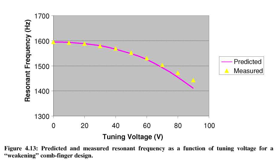

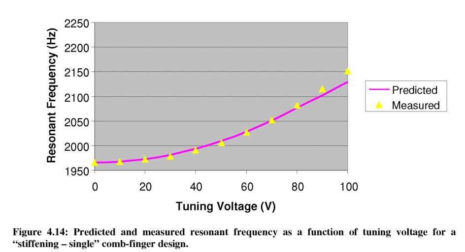
For the “stiffening” resonators, we will first consider the “stiffening - single”

design. The suspension arms are 10p,m wide and the gray-levels were measured to be ~35p,m tall. The extracted k_mech from static tests was 5.7 N/m and an AC drive voltage of 20V was used. Once again, we extract the kelec parameter from FEMLAB simulations and combine it with kmech in Equation 54 to calculate the predicted new resonant frequency. The measured and predicted resonant frequencies agree well and are shown in Figure 4.14. As expected, increasing the tuning voltage causes the resonant peak to shift to higher frequencies, indicating a “stiffening” of keff. SigmaPlot curve fits show that the resonant peak shifted from f₀ = 1965.9 Hz at V_tune = 0 V, to f_tuned = 2151.5 Hz at V_tune = 100 V

Next, we consider the “stiffening - double” design, which according to our simulations, is expected to produce even stronger tuning characteristics. The gray levels were measured to be ~35pm tall, but the suspension width in this case was only 8p.m. Since the suspension spring constant scales with the width (see Equation 47 from Chapter 3), the extracted k_mech from static tests was only 3.2 N/m. Figure 4.15 shows both the measured and predicted resonant frequencies (using FEMLAB simulations and Equations 50 and 54) as a function of tuning voltage. The rapid increase in frequency is larger compared to the “stiffening - single” finger design due in part to the smaller kmech, but also because of the larger kelec produced. SigmaPlot curve fits show that the resonant peak shifted from f₀ = 1332.5 Hz at V_tune = 0 V, to f_tuned = 1560.2 Hz at V_tune = 70 V, a 17% increase in resonant frequency.

4. 

   Tuning Summary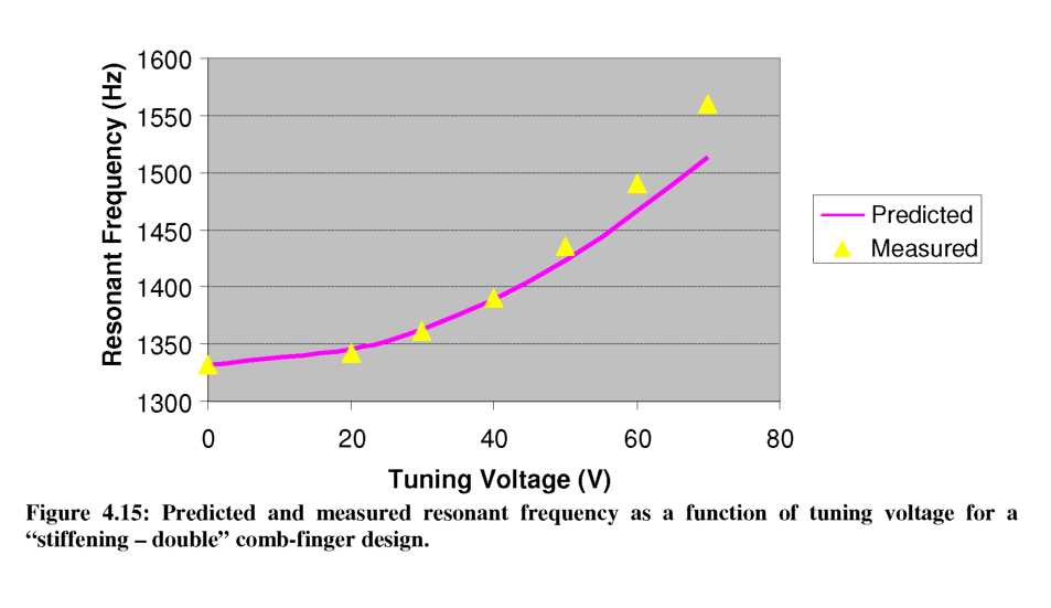

The previous sections have demonstrated multiple tuning configurations for

stiffening and weakening gray-scale comb-finger designs. Since each device is tested separately, and their k_mech and masses are slightly different, it is helpful to compare their extracted k_ei_ec magnitude using Equation 54. Figure 4.16 shows the extracted k_elec for the three gray-scale comb-finger designs, as well as for a planar design where negligible tuning is expected. We see that in each case the measured and predicted values from our model show reasonable agreement, even at high voltages.

For the planar case, we observe a slight spring stiffening effect even though a simplified model of constant height comb-fingers would indicate no electrostatic force gradient there. However, since the resonator layout is asymmetric (with tune fingers only on one side), we should include the capacitor formed by the comb-finger tips. For an order of magnitude estimate, we consider the area created by the comb-finger tips as a parallel plate capacitor, and then use the analysis presented in Equations 50-52. We find that a V_tune = 100 V would produce electrostatic springs on the order of 0.05 N/m, which is ~1/3 of the extracted k_elec for the planar design. We attribute the discrepancy to fringing fields that increase the effective area of the finger tip, causing an underestimation of the capacitive tuning. We believe this small asymmetry also caused a slight stiffening shift in all of designs, as evident from the consistent slight underestimation in the figure.

Figure 4.16: Extracted electrostatic spring constant (k_ei_ec) for the 3 types of gray-scale springs and the planar case for comparison.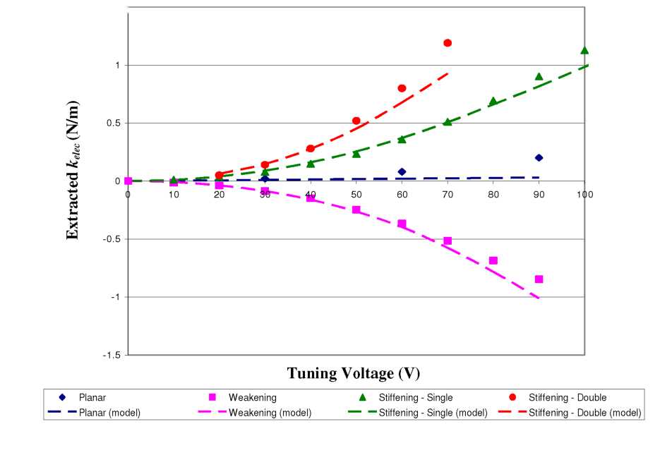

1.5 -]

As expected from our simulations, the strongest relative tuning is achieved with the “stiffening - double” comb-finger design, where an electrostatic spring of 1.19 N/m is created using only 70 V. However, above 70 V, this resonator became unstable due to it’s asymmetric design. Thus, the largest absolute tuning was actually achieved by the “stiffening - single” design since it was able to maintain a stable k_elec up to 120V, resulting in an extracted k_ei_ec of 1.66 N/m. Resonator designs with tuning comb-fingers

on either side of the resonating mass should eliminate any resonator offset induced by the large DC tuning voltages. This would enable the devices to stay in their linear range up to larger tuning voltages; however the versatility and utility of variable-height gray-scale electrostatic springs has been clearly demonstrated.

5. Non-linear Stiffness Coefficients

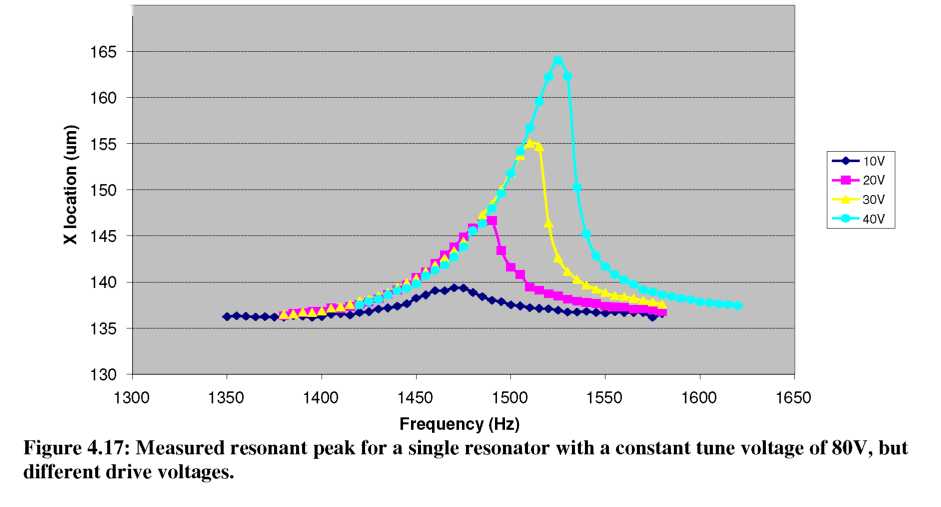
As mentioned in the previous section, the k_ei_ec created by the gray-scale comb- fingers has a limited range over which the spring behaves linearly. Thus, at large deflections or large DC tuning voltages, the presence of non-linear stiffness coefficients becomes important. An example of this non-linear behavior for the “weakening” resonator design presented earlier is shown in Figure 4.17 (un-tuned /0=1594.6 Hz). For each of the 4 cases shown, the tuning voltage was held constant at 80V, but the amplitude of the drive signal was changed from 10V to 40V. At the lowest drive voltage of 10 V, the tuned resonant frequency was 1472.5 Hz. In a linear system, the peak should simply change height as driving amplitude changes. However, the figure shows that large drive amplitudes cause the peak to bend/creep towards the original f₀.

170 -|

In general, such a system can be described by the Duffing equation [146]:

mx + £x + kx + yc³ = b cos(at) (58)

where £, is the damping coefficient and у represents a third-order term in the spring constant, such that:

F = kx ±\Yx³. (59)

Exact solutions to the Duffing equation are not, in general, available [138], but the concept of both “hard” (y>0) and “soft” (y<0) springs are shown in Figure 4.18. In some frequency ranges, multiple stable solutions exist and the resonator may ‘jump’ from one position to the next as the frequency changes [138], an undesirable effect in most cases.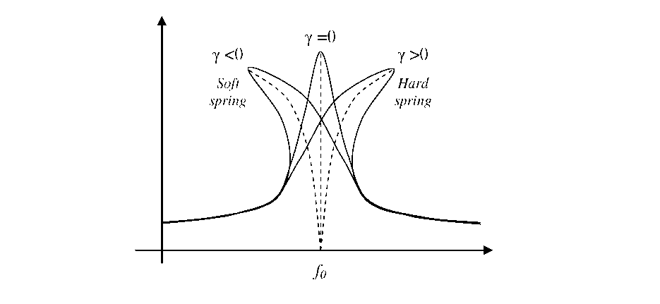

Figure 4.18: Schematic of frequency response for a resonator with non-linear stiffness coefficients.

For a typical un-tuned resonator, as the resonant amplitude increases, cubic stretching terms in the suspension spring constant [147, 148] can become non-trivial, leading to a “hard” spring behavior [138, 146]. Parallel plate electrostatic springs have been found to exhibit “soft” spring behavior [146], an inherent artifact of their cubic dependence on amplitude and gap from Equation 52.

In contrast, the tendency of vertically shaped resonators developed in this work is to bend towards the original f₀ (i.e. a “weakening” design shows “hard” spring behavior and a “stiffening” design shows “soft” spring behavior). This occurs because kelec at the rest position is typically at a peak value, so large vibrations move the resonator to regions of significantly lower k_elec and the amount of tuning decreases.

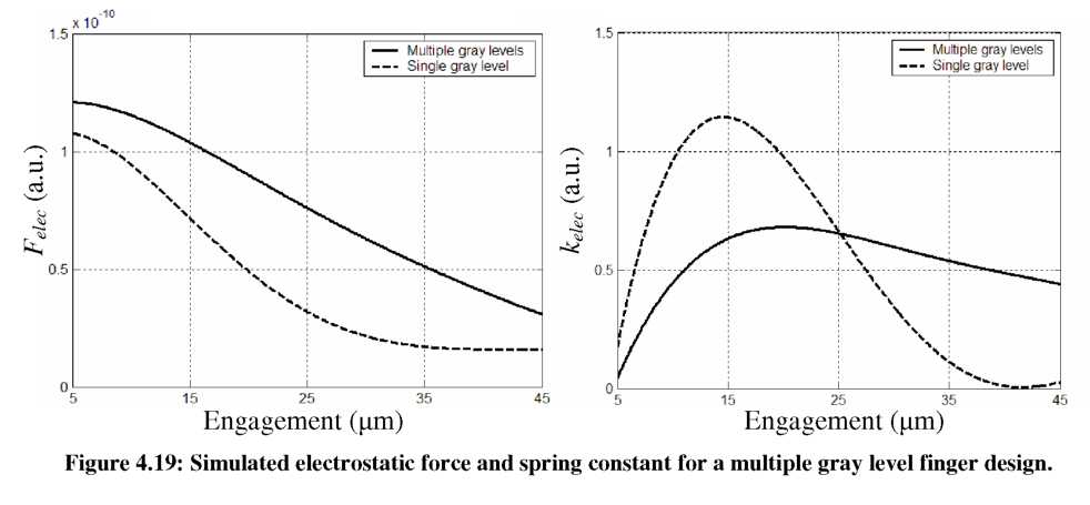
Two potential methods will now be presented to deal with these non-linear effects. First, multiple gray levels can be used to further tailor the capacitance profile to extend the linear range of the electrostatic spring. For example, Figure 4.19 shows the simulated electrostatic force and spring constant for a single gray level design (“stiffening - single,” 10p,m tall) compared to a multi-gray level design (three additional 10p,m long intermediate steps with heights of 70p,m, 50p,m, and 30p,m). As evident from the figure, the single gray level design provides a steep change in force over a short distance. The multi-gray level design provides the same total change in force, but it now takes place over a large engagement distance, leading to a slightly smaller spring constant that is more consistent with engagement.

Complex force-engagement profiles could be developed through simulation to tailor spring behavior, though the simulation process is quite slow. However, a second method for extending the linear range of electrostatic springs is also briefly introduced below. By staggering the relative engagement of single-gray level comb-fingers, by 5 as shown in Figure 4.20, the sum of appropriately spaced electrostatic springs could be used to create a wide linear range of operation. In this case, a single gray level design can be simulated accurately in 3-D FEA and the result manipulated easily within a simpler programming language (such as MATLAB).

Figure 4.20: Schematic of a variable-engagement comb-finger design.

To investigate this concept in more depth, we start by considering the simulated spring constant as a function of engagement for a single finger, as done previously in Figure 4.6 - Figure 4.8. We then use the sum of many staggered fingers to create an arbitrary k_elec-engagement profile:

where ko(x) is the k_elec-engagement profile of a single un-shifted finger and 5_n is the shift of each individual finger. For the simplest case of shifting A fingers forward and B fingers backward by an identical amount, we have:

Thus, the problem has reduced to simply finding two coefficients, A and B, which determine the relative number of comb-fingers with each shift (+5o or -5o).

For example, Figure 4.21 shows a simulated electrostatic spring without any offset, where the magnitude of kelec changes dramatically with engagement. However,

when an offset of 5₀=8pm is used (with A = 5g and B = 38), a plateau >20pm wide is

created where there is negligible change in kelec. Thus, a tunable resonator with 48 fingers (like before) would be designed with 30 fingers shifted forward and 18 fingers shifted backward from a neutral point. More complicated combinations of offsets and coefficients could be used to extend and/or tailor the k_elec-engagement profile as desired. In some instances, this manipulation of high-order stiffness coefficients may prove useful for purposes beyond improving linearity (such as incorporating “soft” electrostatic springs to compensate for “hard” mechanical spring behavior due to material stretching).