3. Gray-scale Electrostatic Springs

The design, simulation, and fabrication of variable height gray-scale electrostatic springs used here are quite similar to the methods developed in Chapter 3. The following sub-sections will introduce the three types of variable-height electrostatic springs investigated in this research, as well as simulation and fabrication results to predict their relative spring constants.

1. Design

As evident from simulations in Chapter 3, a vertical step in comb-finger height creates a smoothly varying force-engagement profile (see Figure 3.9), of which a portion appears to be quasi-linear and could be used an electrostatic spring. Therefore, the three designs presented here contain only a single gray level for simplicity, and the height of the gray level (in conjunction with the applied voltage) will determine the strength of the electrostatic spring. More precise force-engagement profiles are possible by incorporating more gray levels (as will be shown with simulations in Section 4.5).

The first gray-scale electrostatic spring design is shown in Figure 4.4, where the moving comb-fingers initially engage with a reduced height section, followed by a full height (planar) section. Such a design is analogous to the decreasing gap design shown in Figure 4.2, and will thus be referred to as the “weakening” finger design.

A second electrostatic spring design is shown in Figure 4.5(a). The moving finger initially engages with a full-height (planar) section, followed by a reduced height section some distance later. Thus, the electrostatic force decreases as the engagement increases, analogous to an increasing gap comb-drive design. The net effect is a “stiffening” of keff.

2. 

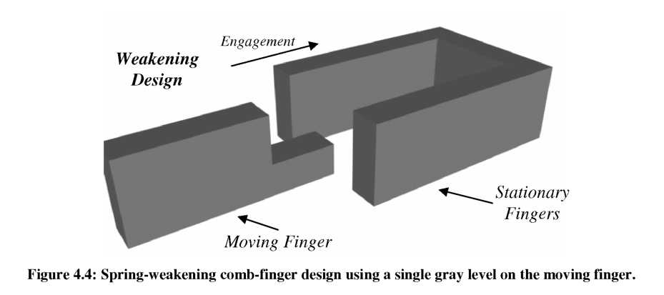
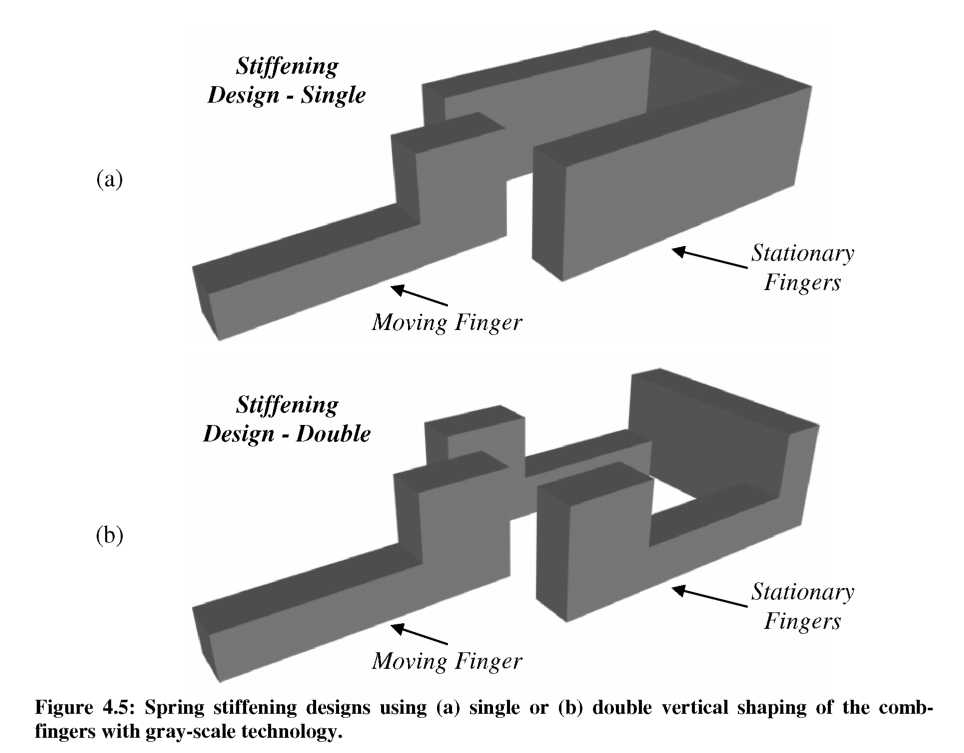
   Figure 4.5(b) shows an additional novel design that vertically-shapes both stationary and moving comb-fingers. As the fingers engage in this “stiffening - double” design, there should be a dramatic change in force as the two full-height sections pass each other. Since the fully engaged force will be lower for the “double” design, it is anticipated that a more dramatic electrostatic spring “stiffening” effect will be observed (assuming the change in force from max to min occurs over a similar engagement change). A variable-gap comb-finger design would have particular difficulty replicating the analog to this “double” shaping design since it would require shaping both moving and stationary fingers, leading to an increase in device footprint. It must be noted that the electrostatic spring will be non-linear for each of these three cases due to their simplistic design, a trait that will be discussed in more detail towards the end of this chapter.

   Simulation

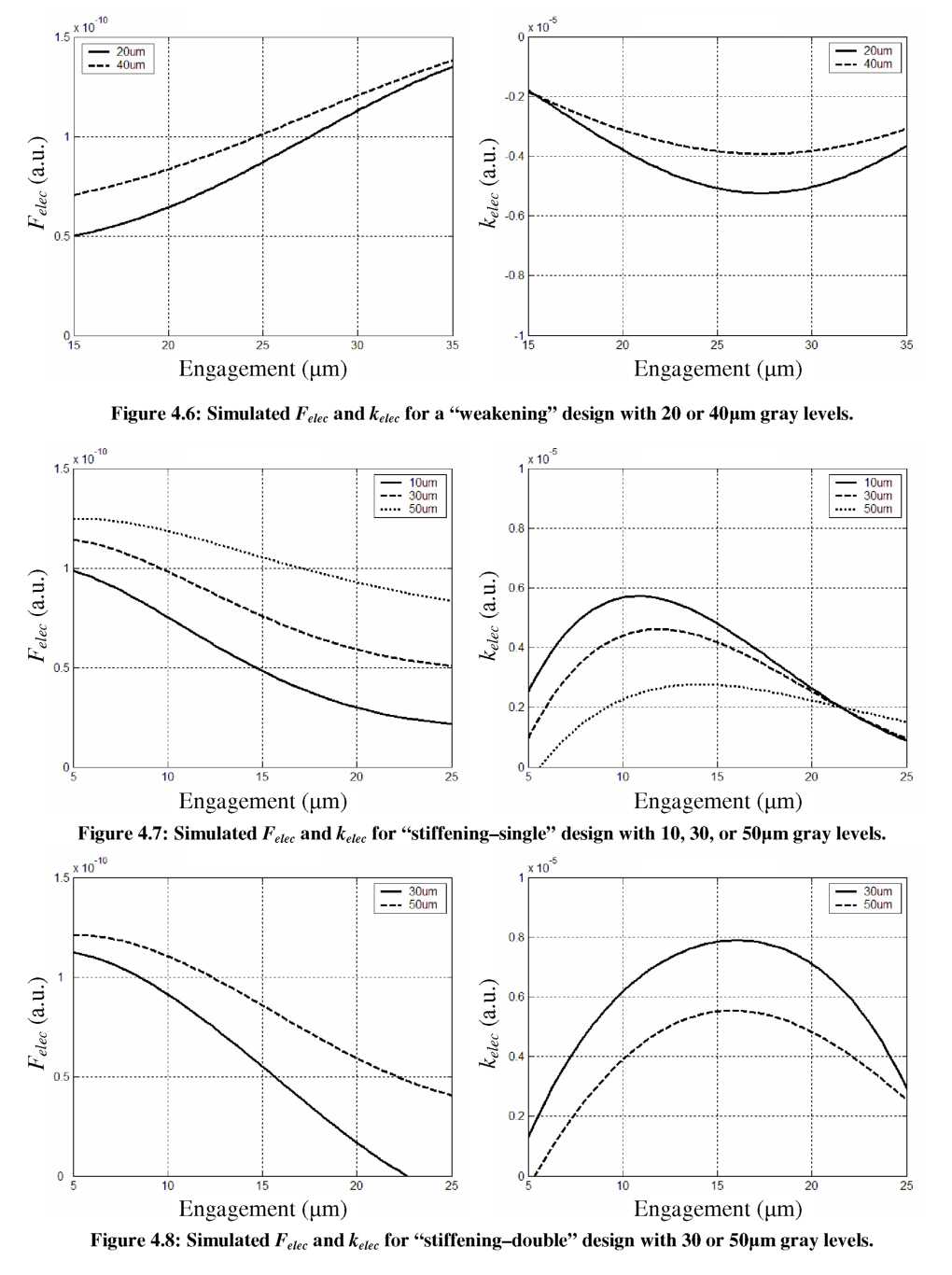
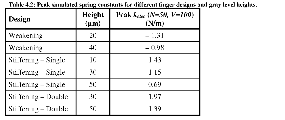
The capacitance as a function of engagement for each spring design was

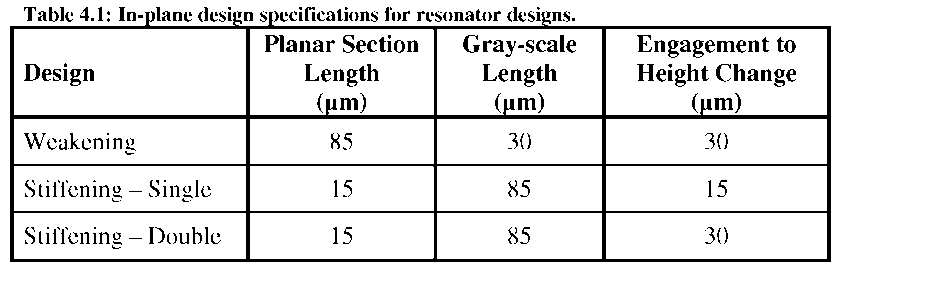
simulated using FEMLAB for different gray level heights. As in Chapter 3, 100p,m SOI wafers are assumed, with 10p,m comb-finger gaps and widths. Capacitance-engagement data were fit with a 6^th-order polynomial, and the derivative taken near the height change to obtain the local force-engagement profile. The horizontal geometry of each design and the engagement required to reach the edge height step(s) are shown in Table 4.1.

A derivative of the force-engagement profile near the height step was used to estimate the generated electrostatic spring constant. While in general taking multiple derivatives of polynomial fit functions can be inaccurate, later results will show that derivatives in the middle of the simulated range (near the height step) are able to predict resonator behavior with reasonable accuracy. Plots of the 1^st and 2^nd derivatives of the simulated capacitance for each type of comb-finger design are shown in Figure 4.6, Figure 4.7, and Figure 4.8, where each line indicates a specific height of the associated gray level. The plots represent example electrostatic forces (Felec - left plots) and spring constants (kelec - right plots) as a function of engagement for a single comb-finger.

The 1^st derivative of capacitance can be used in Equation 26 from Chapter 3 to obtain the force, while the 2^nd derivative should be plugged into Equation 50 from Chapter 4 to obtain the spring constant. In each case, one must multiply by the number of comb-fingers in the system. The peak value of k_elec is calculated in Table 4.2 for each simulated design, assuming N=50 comb-fingers and an applied voltage of 100V. As expected, lower gray levels create larger changes in force, and thus higher magnitudes of k_elec. It is also clear that the “stiffening - double” design is a significant improvement over the “stiffening - single” design (1.97 N/m vs. 1.15 N/m for 30p,m high gray levels).

As a rough comparison, we consider the geometry required for a planar, variable- gap model to produce tuning equivalent to the “stiffening - double” design above (using the model of Jensen et al [61]). For similar fabrication constraints, the gap would have to change from approximately 10p,m to 20p,m over a 10p,m engagement length. However, by changing the gap, the density of fingers is reduced, so a device with similar footprint will only provide 2/3 the tuning of the gray-scale devices shown above. It is possible that a combination of variable-gap and variable-height comb-fingers could provide even stronger tuning effects.

3. Layout and Fabrication

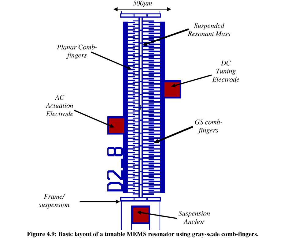
The layout of tunable gray-scale resonators is based on that shown in Figure 4.9.

A set of 48 stationary planar comb-fingers are connected to an actuation electrode, where the AC drive signal is applied. The “tune” electrode on the right side, which always receives a DC voltage, is attached to 48 stationary gray-scale comb-fingers. The resonant mass is made entirely of planar comb-fingers, except for the “stiffening - double” design that requires comb-fingers on the “tune” side of the resonant mass to be shaped vertically.

The design above was developed for simplicity, however there is an obvious asymmetry of applied forces. While a small (~20V) AC signal will be used on the left side to drive the resonator, DC tuning voltages up to 100 V will be applied to the tune

electrode on the right side to maximize kelec. This bias will cause the device to resonate around a deflected point (5-10p,m). Since k_elec is position dependent in Figures 4.6-4.8, static deflections will effect the magnitude of the electrostatic spring. To anticipate these offsets, the rest position of the comb-fingers was biased so that the peak kelec occurs after ~5p,m of deflection.

All resonator devices were fabricated using the SOI gray-scale actuator process described in Chapter 3. The approximate measured gray level height for each type of device tested in the following section is shown below in Table 4.3. For comparisons with the models presented earlier above, the simulated value closest to the measured height will be used for kelec predictions.