
- •1.The role of Microeconomics
- •2. T he Subject Matter of Microeconomics
- •3. The use and limitation of Microeconomic theory
- •4. Economic methodology and microeconomic models
- •5. Equilibrium analysis
- •6. Positive and normative analysis
- •7. Demand Function(df): Individual df vs Market df
- •8. Change in Quantity Demanded, Change in Demand
- •9.Inferior, Normal and Superior Goods
- •10. Supply Function. Change in quantity supplied and Change in supply
- •11. Market equilibrium
- •12 Market Adjustment to Change: shifts of Demand and shift of Supply
- •Shifts of Demand
- •13. Changes in Both Supply and Demand
- •14. Cobweb theorem as an illustration of stable and unstable equilibrium
- •Unstable cobweb
- •Constant cobweb
- •15. Government regulation of a market
- •1. Price ceiling and Price floor
- •2. Impact of a tax on price and quantity
- •16. Price ceiling and Price floor
- •Impact of a tax on price and quantity
- •18. Demand elasticity. Price Elasticity Coefficient and Factors affecting price elasticity of demand
- •Table of price elasticity kinds of demand
- •19. Impact of demand elasticity on price and total revenue
- •20. Income elasticity of demand(yed)and Cross elasticity of demand
- •Categories of income elasticity:
- •21. The price elasticity of supply
- •22. Market adaptation to Demand and Supply changes in long-run and in short-run
- •24.Consumer Choice and Utility
- •25. Total Utility (tu) and Marginal Utility (mu)
- •26. Indifference curves.
- •28. The effects of changes in income and prices
- •29 Equimarginal Principle and Consumer equilibrium
- •30.Income Consumption Curve. Engel Curves
- •32. Income and Substitution Effects
- •The slutsky method
- •34. Production Function
- •35. Time and Production. Production in the Short-Run
- •36.Average, Marginal and Total Product. Law of diminishing returns
- •37. Producer’s behavior
- •38 Isoquant
- •39. Isocost
- •40. Cost minimization (Producer’s choice optimisation)
- •41.The treatment of costs in Accounting and Economic theory
- •Average costs. Marginal Cost
- •Long run average cost. Returns to Scale.
- •45Different market forms
- •48 The Competitive Firm and Industry Demand
- •49.Economic strategies of the firm in p-competitive m arket
- •50.Long run equilibrium
- •51.Definition of Monopoly Market. Causes of monopoly.
- •Patents and Other Forms of Intellectual Property
- •Control of an Input Resource
- •Capital-consuming technologies
- •Decreasing Costs
- •Government Grants of Monopoly
- •52.Monopoly Demand and Marginal Revenue
- •54. Monopoly Inefficiency
- •Negative consequences of Monopoly
- •55. "Natural" Monopoly
- •Government Ownership
- •56. Imperfect competition and Monopolistic competition
- •57. Profit Maximization in Monopolistic Competition
- •58. Oligopoly
- •59. Firms behavior in Oligopoly
- •60 Kinked Demand Model
- •61 Competitive factor markets
- •62 The Demand for Inputs
- •63 Supply of Inputs
- •64. Equilibrium in a Market for Inputs
- •Labour market
- •Land market
- •Capital market
- •65. Labor market: labor demand and supply of labor.
- •66.The Marginal productivity approach to demand for labor.
- •Equilibrium and disequilibrium on labor market.
- •68. Particularities of Land market. Differential rent. Marginal productivity of land.
- •69 Main characteristics of Asset market. Demand for capital. Interest rate.
- •70. Discounted value. Conceptions of Net present value (npv) and future present value (fv).
- •The role of Microeconomics
- •T he Subject Matter of Microeconomics
64. Equilibrium in a Market for Inputs
Labour market
The price of labor is the wage(w), and the quantity demanded is the number of labor-hours employed(L). The demand for labor is the MRP, the price of output times the marginal productivity of labor in units of output. As usual, the equilibrium price (wage) and the equilibrium quantity demanded and supplied (employment) are at the point where the supply and demand curve intersect.
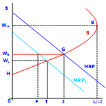
Figure 3: Supply and Demand for Labor
Land market
Land is not a homogenous resource, and that important complication cannot be skipped over. It is the basis of the theory of rent(land is more fertile than other kinds of land, or more profitable because it is closer to markets; and some land is more suitable to one kind of crop than another). These differences in fertility will be reflected in the marginal productivities and therefore in the demands for the different kinds of land.
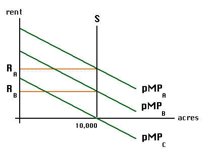
: Marginal Productivity of Land with Different FertilitiesThe demand for good land is pMPA, for fair land pMPB, and for bad land pMPC. Supply of land of a particular quality is always a vertical line, because "they're not making any more of it" – the supply of land cannot be increased no matter how high the price. Since there are 10,000 acr. of each sort of land, three kinds of land have identical supply curves,all shown by the vertical line S.
In a supply-and-demand equilibrium, then, the rent per acre of good land will be RA. For fair land it will be RB, and for bad land zero.
Thus, the rent on fair land is just enough to offset its greater productivity relative to the marginal land. Similarly, the rent on good land is just enough to offset its productivity advantage over marginal land.The difference in rent between the good and fair land is just enough to offset the productivity differential between them. This is called the "differential" theory of rent – that the rent of any land is just large enough to offset its differential productivity relative to marginal land. To stress the basis of land rent, it is often called differential rent.
Capital market
As we increase the number of machines in use, with the same amount of land and labor, output will increase, but at a decreasing rate. Capital is subject to diminishing returns. Once again, we will focus on the "marginal productivity" of the machines. On the other hand, the costs of using the machinery will also increase as the number of machines increases. We assume that the firm uses a given quantity of labor and land and that the quantity of capital used varies. The quantity of capital used (measured in dollars' worth) is marked off on the horizontal axis. On the vertical axis is the rate of interest, which we understand as the price of capital.
The horizontal red line is the supply curve of capital to the firm, green-demand for capital, that is, the marginal productivity of capital (net of the cost of wear and tear of specific capital goods) times the price of the output – the value of the marginal product of capital. The profit-maximizing demand for capital for the firm is shown by K. That is, it will be profitable to expand the capital stock of the company until diminishing returns reduces the value of the marginal product to r, the market rate of interest, at K.