61 Competitive factor markets

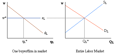
Factor markets are much like output markets, but with one important difference. The demand for factors is a derived demand. For example, a firm's demand for labor depends upon how much output the firm will produce. More output leads to a greater demand for laborers, less output leads to a lower demand for laborers. Consider the case where there is one variable factor called labor and that this labor is bought and sold in a competitive labor market. The use of the term competitive designates a situation that is similar to what we would find in a competitive output market. In this case, each buyer of labor is one of many buyers in the market. The labor market determines the wage facing individual buyers, who purchase as many workers as needed at the given wage rate. As a result, the supply of labor facing any individual buyer is a horizontal line at the going wage rate. The graph below shows this.

The quantity of labor hired by each firm depends on where the marginal benefit of each hired factor equals the cost of hiring that factor. The marginal benefit (MB) is given by how each extra laborer affects the firm's revenues, whereas the marginal cost (MC) of each additional laborer is how each laborer affects the firm's total costs. In equation form, MB and MC are given as: MB = DTR/DL

MC = DTC/DL Because firms can hire as many workers as needed at the existing wage rate, we know that the second equation (which describes the supply of labor) can be rewritten as MC = w. The first equation (which gives us the demand for labor) can be rewritten as: MB = (DTR/DQ)(DQ/DL). That is, the marginal benefit of hiring additional workers is the product of a firm's marginal revenue and marginal product of labor. Note that marginal revenue is determined by the firm's output decision in the output market, while marginal product is determined by the firm's hiring decision in the factor market. Because a firm's marginal revenue curve depends on the market structure of the output market, the firm's demand for labor will depend on the market structure in the output market as well. For example, if a firm operates in a perfectly competitive output market, then the firm's marginal revenue is equal to the market price. If a firm is a monopolist in the output market, then the firm's marginal revenue is less than the price. Let's compare the demand for labor between a perfectly competitive industry and a monopoly that operate in identical output markets. Assume that both industries draw from the same labor market (e.g. the unskilled labor market) and that there are many other firms doing the same thing. The demand for labor by firms in any industry is the product of marginal revenue and the marginal product of labor. Perfectly competitive firms have a marginal revenue that equals the market price (i.e. MR = P). If MR = P, then we can rewrite the demand for labor by firms in a perfectly competitive industry as (P x MP_L). This term can be refered to as the marginal value product of labor (MVP_L). Monopolists produce where their marginal revenue is less than the market price. Therefore, we cannot rewrite the monopolist's demand for labor as (P x MP_L). The monopolist will have a demand for labor equal to (MR x MP_L), which we call the marginal revenue product of labor (MRP_L).