Government Grants of Monopoly

Monopolies can be created by legislation. Historically, this has been an important source of monopolies as, for example, a monarch might grant a monopoly of wine to a favorite. In the modern world, governments may still encourage monopoly in many countries of the world, though this seems less common as time goes on.

52.Monopoly Demand and Marginal Revenue

The demand curve for the monopoly is the demand curve for the industry – since the monopoly controls the output of the entire industry – and the industry demand curve is downward sloping. So the monopoly's demand curve is downward sloping. That means the monopoly can push the price up by limiting output. If the monopoly cuts back on its output, it can move up the industry demand curve to a higher price.

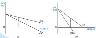
Figure 2 shows that the MR curve lies below the AR curve. We can conclude that if the AR curve (i.e. the demand curve) is falling steeply, the MR curve is far below the AR curve. On the other hand, if the AR curve is less steep, the vertical distance between the AR and MR curves is smaller. Figure 2 (a) shows a flatter AR curve while Figure 2(b)

shows a steeper AR curve. For the same units of the commodity, the difference between AR and MR in panel (a) is smaller than the difference in panel (b).

The MR values have a relation with the price elasticity of demand. It is sufficient to notice only one aspect – price elasticity of demand is more than 1 when the MR has a positive value, and becomes less than the unity when MR has a negative value. As the quantity of the commodity increases, MR value becomes smaller and the value of the price elasticity of demand also becomes smaller. Recall that the demand curve is called elastic at a point where price elasticity is greater than unity, inelastic at a point where the price elasticity is less than unity and unitary elastic when price elasticity is equal to 1.

53. Monopoly Profit Maximization

The profit received by the firm equals the total revenue minus the total cost. In the figure, we can see that if quantity q1 is produced, the total revenue is TR1 and total cost is TC1. The difference, TR1 – TC1, is the profit received. The same is depicted by the length of the line segment AB, i.e., the vertical distance between the TR and TC curves at q1 level of output. It should be clear that this vertical distance changes for diferent levels of output.

When output level is less than q2, the TC curve lies above the TR curve, i.e., TC is greater than TR, and therefore profit is negative and the firm makes losses.

The same situation exists for output levels greater than q3. Hence, the firm can make positive profits only at output levels between q2 and q3, where TR curve lies above the TC curve. The monopoly firm will choose that level of output which maximises its profit. This would be the levelof output for which the vertical distance between the TR and TC is maximum and TR is above the TC, i.e., TR – TC is maximum. This occurs at the level of output q0. If the difference TR – TC is calculated and drawn as a graph, it will look as in the curve marked ‘Profit’ in Figure 3. It should be noticed that the Profit curve has its maximum value at the level of output q0.

The analysis shown above can also be conducted using Average and Marginal Revenue and Average and Marginal Cost. Though a bit more complex, this method is able to exhibit the process in greater light.

In Figure , the Average Cost (AC), Average Variable Cost (AVC) and Marginal Cost (MC) curves are drawn along with the Demand (Average Revenue) Curve and Marginal Revenue curve.

The rule for monopoly profit maximization will come as no surprise. It is

MR=MC

That is, the rule says that the monopoly should increase output up to the level where the marginal cost curve intersects the marginal revenue curve, in order to maximize its profits. The price charged is the corresponding price on the demand curve. Notice that this is a two-stage analysis:

• at the first stage, the marginal cost and the marginal revenue determine the output. Profit maximizing output is the output at which they intersect.

• at the second stage, the output and the demand curve determine the price. Trace up the vertical line to the demand curve, and that's the profit-maximizing price.

Thus, a profit-maximizing monopoly will sell less than the supply-demand output, at a higher price.