48 The Competitive Firm and Industry Demand

The individual firm's demand curve is different from that of the industry, and is more elastic. This is because substitutes increase elasticity, and the customer of the firm has many good substitutes for that firm's output – namely, the output of other firms in the industry. As we mentioned above, the demand curve for a P-Competitive firm is infinitely elastic:

In the figure, the lower case q, s and d refer to output, supply and demand from the point of view of the individual firm, respectively, and the capital S, D, and Q are for the industry as a whole.

49.Economic strategies of the firm in p-competitive m arket

H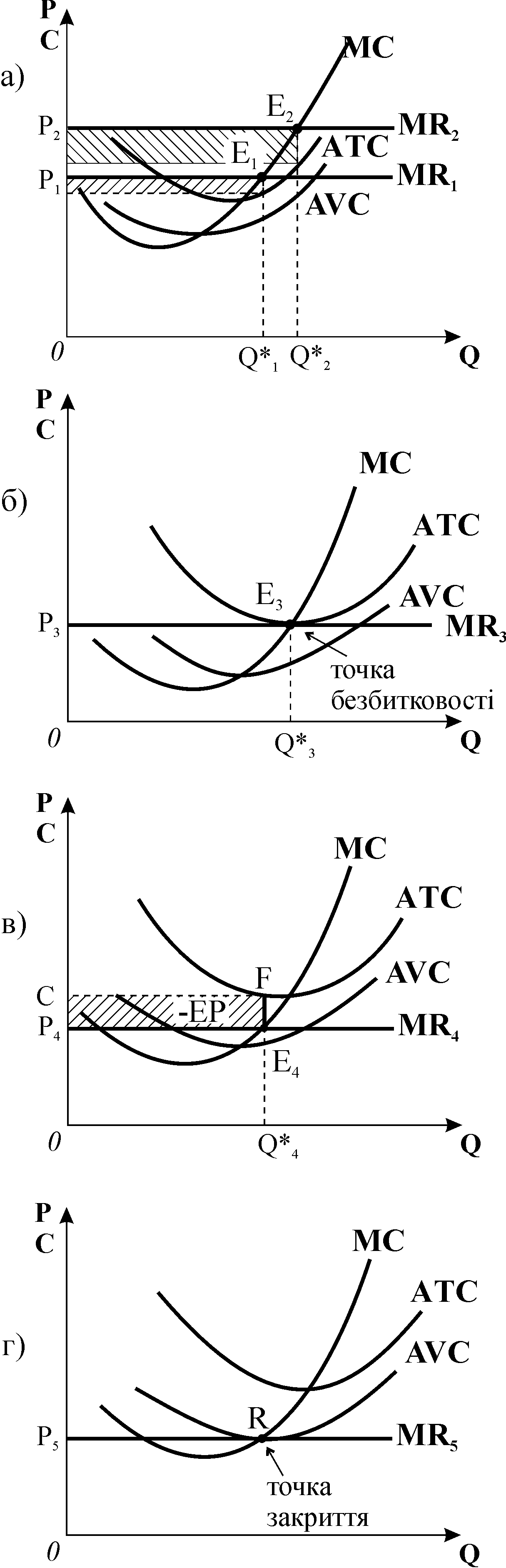 ow much output should firm sell, at the given price to maximize profits. The answer is: increase output until P=MR=MC

Now we will use this rule as a basic rule to consider the firm economic strategies.

In the picture just shown, the firm is making an "economic profit." All costs, explicit and implicit, are included in the firm's Average Cost curve.

Profitableness and losses conditions for perfect competitor according to MRMC-model:

a) a firm has profit under:

б) break-even condition is:

в) losses minimization condition through production continuance:

г )losses minimization condition through temporary dissolution of the firm:

In other words if the cost of and additional unit (MC) is less than the revenue obtained from that same additional unit (MR), producing the additional units will add to profits (or reduce losses). If the cost of additional units of output (MC) cost more than they add to revenue (MR), the firm should not produce the additional units. The rules for profit maximization are simple:

• MR >MC – produce it!

• MR < MC – don’t produce it!

• When MR = MC – you are earning maximum profits!

MR=MC is the main principle of supply for the individual firm. Supply is the relation between the price and the quantity that people want to sell. For an individual firm, that is: the relation between the price and the quantity the firm wants to sell. So we ask: at a given price, how much will a (profit- maximizing) firm want to sell? The answer: enough so that the price is equal to marginal cost. In other words, the marginal cost curve is the supply curve for the individual firm.

50.Long run equilibrium

Profit opportunities will attract new firms into the industry. With "free entry," the (short run) supply curve of the industry shifts to the right, causing the price to drop until the economic profits are eliminated.

This process of entry and price change is known as the "long run equilibrium process" and it continues until "long run equilibrium" is attained. Here is a picture of the firm and industry in "long run equilibrium:"

The new price, quantity, firm demand and short run supply are indicated by primes -- p', q'. Q', d', S'. We see that, at a slightly lower price, the individual firm is lower on the MC curve and produces a little less, but since there are more firms in the industry, the industry as a whole produces more.

We notice something else about the long-run equilibrium of a P-Competitive industry: each firm chooses the plant and equipment and productive capacity that gives the lowest average cost overall. This is shown by the above figure.

To see what this means, we might ask the following hypothetical question:

If an industry is to produce a certain amount of output, how should the output it be divided up among the different firms? More specifically, how many firms should share that production assignment? If there are very many firms, then each will be producing at a very small scale. They will not be taking advantage of the economies of scale, and cost per unit will be high. On the other hand, if there are very few firms, each will be producing on a very large scale, and suffering from diseconomies of scale, so, again, unit costs would be high. It would be best to balance the disadvantages of too large scale against the disadvantages of too small scale, and have just enough firms in the industry so that each is at the bottom of its average cost curve. The total cost of producing that output is then at a minimum.

We have seen that profits will lead to the entry of new firms into a P-competitive industry. This also works in the opposite direction: if firms in the industry were taking losses, supply in the industry will decrease. Firms in the industry might continue to produce in the short run, despite the losses. Remember that a profit-maximizing firm will continue to produce, in the short run, so long as it can cover its variable costs. However, in the long run, firms will drop out of the industry, if they continue to lose money. Thus, the supply curve of the unprofitable industry will shift to the left. But that in turn means prices will rise, and the long run equilibrium comes where the price is equal to average cost.

This discussion could apply to any economic activity to which there is "free entry." Economic profits – profits over and above the opportunity cost of capital – will attract new entrants. Returns less than the opportunity cost of capital will cause firms to get out of the industry. This will continue until the return to capital in that activity is the same as the opportunity cost of invested capital, that is, until profits are zero. We might call this principle "the Entry Principle". It says that in the long run, with free entry, returns to invested capital in an industry are just enough to offset the opportunity cost. When there are economic profits or losses, entry into the industry or exit of firms from it will shift the industry supply until economic profits are zero.