

Average costs. Marginal Cost
Average fixed cost (AFC) This is the quotient of fixed cost divided by output.
Average variable cost (AVC) This is the quotient of average cost divided by output.
Average total cost (ATC or AC) This is the quotient of total cost divided by output.
The average fixed costs decline as the fixed costs are "spread over more units of output." For large outputs, however, average variable costs rise pretty steeply. ." The average total cost, dominated by fixed costs for small output, declines at first, but as output increases, fixed costs become less important for the total cost and variable costs become more important, and so, after reaching a minimum, average total cost begins to rise more and more steeply.
Marginal
cost is defined as:
![]()
As
usual, Q stands for (quantity of) output and C for cost, so
![]() Q
stands for the change in output, while
C
stands for the change in cost. As usual, marginal
cost
can be interpreted as the additional cost of producing just one more
("marginal") unit of output.
Q
stands for the change in output, while
C
stands for the change in cost. As usual, marginal
cost
can be interpreted as the additional cost of producing just one more
("marginal") unit of output.
This
is a good representative of the way that economists believe firm
costs vary in the short run:
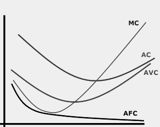
The output produced is measured by the distance to the right on the horizontal axis. The marginal cost rises to cross average cost at its lowest point.
The point is illustrated by the following table, which extends the marginal cost table in an earlier page to show the price and the profits for the example firm.
Long run average cost. Returns to Scale.

Therefore, the long run average cost (LRAC) – the lowest average cost for each output range – is described by the "lower envelope curve," shown by the thick, shaded curve that follows the lowest of the three short run curves in each range.
More realistically, an investment planner will have to choose between many different plant sizes or firm scales of operation, and so the long run average cost curve will be smooth, something like this:
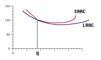
As shown, each point on the LRAC corresponds to a point on the SRAC for the plant size or scale of operation that gives the lowest average cost for that scale of operation.
Returns to Scale The cost per unit changes as the scale of operation or output size changes. Here is some terminology to describe the changes:
average cost decreases as output increases in the long run = increasing returns to scale = decreasing cost
average cost is unchanged as output varies in the long run = constant returns to scale = constant costs
average cost increases as output increases in the long run =decreasing returns to scale = increasing costs
Here are pictures of the average cost curves for the three cases:
1 .
Increasing returns to scale = decreasing cost
.
Increasing returns to scale = decreasing cost
It is necessary to use less productive methods to produce the smaller amounts. Thus, costs increase less than in proportion to output – and average costs decline as output increases.
Increasing Returns to Scale is also known as "economies of scale" and as "decreasing costs."
2. Constant returns to scale = constant costs
O ne
machinist used one machine tool to do a series of operations to
produce one item of a specific kind - and to double the output you
had to double the number of machinists and machine tools.
Constant
Returns to Scale is also known as "constant costs.
ne
machinist used one machine tool to do a series of operations to
produce one item of a specific kind - and to double the output you
had to double the number of machinists and machine tools.
Constant
Returns to Scale is also known as "constant costs.
3. Decreasing returns to scale = increasing costs
Decreasing
returns to scale are associated with problems of management of large,
multi-unit firms.
. Decreasing Returns to Scale is also known as "diseconomies of scale" and as "increasing costs".