38 Isoquant

A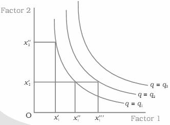 n isoquant is the set of all possible combinations of the two inputs that yield the same maximum possible level of output. Each isoquant represents a particular level of output and is labelled with that amount of output. Cobb-Douglas Isoquants

An isoquant plots all the combinations of two inputs that will produce a given output level. A point on the isoquant curve is technically efficient.In general, isoquants are downward sloping – the more labor we use, the less capital we need. It is bowed inward because of the law of diminishing marginal productivity. In the case of Cobb-Douglas Isoquants inputs are not perfectly substitutable. The slope of an isoquant shows the rate at which L can be substituted for K.

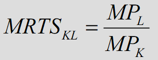
- slope = marginal rate of technical substitution (MRTS). RTS > 0 and is diminishing for increasing inputs of labor. The marginal rate of technical substitution (RTS) shows the rate at which labor can be substituted for capital while holding output constant along an isoquant:

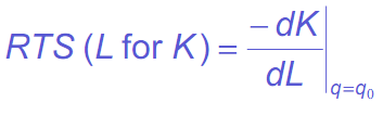or

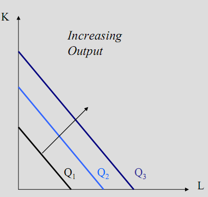
Isoquant map – a set of isoquant curves that show technically efficient combinations of inputs that can produce different levels of output. Leontief Isoquants

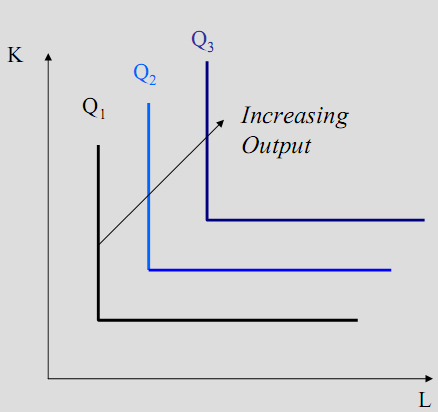K and L perfect substitutes perfect complements

39. Isocost

Isocost line – a line that represents alternative combinations of factors of production that have the same costs. Or in other words, the combinations of inputs (K, L) that yield the producer the same level of output.

The shape of an isoquant reflects the ease with which a producer can substitute among inputs while maintaining the same level of output.

The combinations of inputs that produce a given level of output at the same cost can be expressed as:

wL + rK = C

Rearranging, K= (1/r)C - (w/r)L

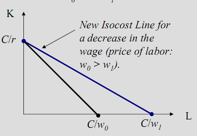
For given input prices, isocosts farther from the origin are associated with higher costs

Changes in input prices change the slope of the isocost line

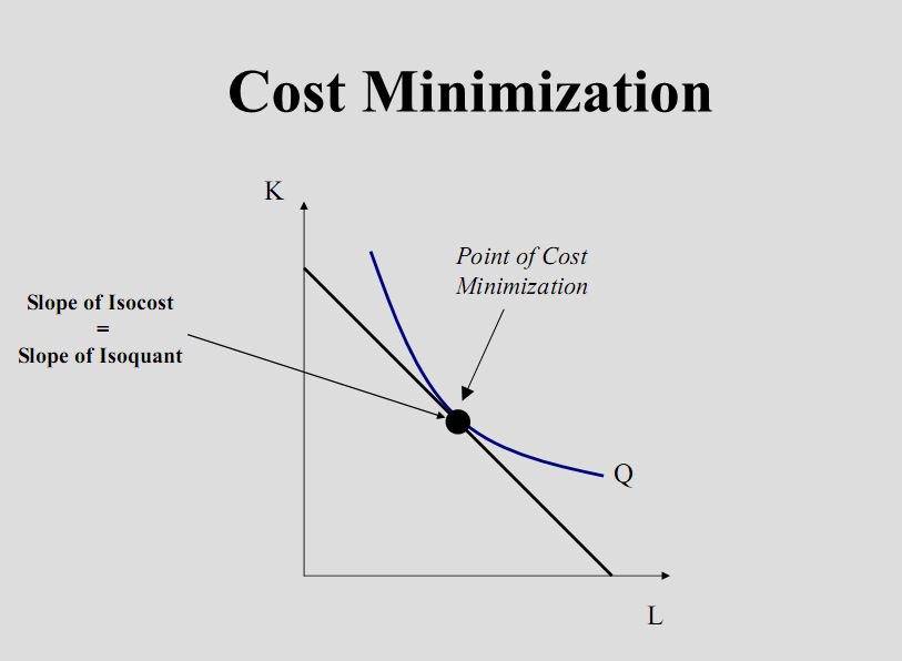
40. Cost minimization (Producer’s choice optimisation)

The least cost combination of inputs for a given output occurs where the isocost curve is tangent to the isoquant curve for that output.

The slopes of the two curves are equal at that point of tangency.

The firm is operating efficiently when an additional output per dollar spent on labor equals the additional output per dollar spent on machines.So that marginal product per dollar spent should be equal for all inputs:

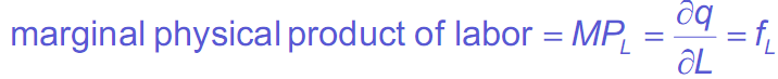
We define marginal physical product as the additional output that can be produced by employing one more unit of that input while holding other inputs constant:

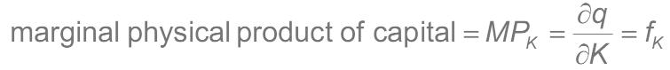
and

Choosing the Economically Efficient Point of Production can be shown in the graph:

41.The treatment of costs in Accounting and Economic theory

The production relationships and prices of inputs determine costs. The price of the factor for the firm is the cost (the amount of money spent to get the factor). Accountants traditionally considered only money costs. Wages, expenditure on raw materials, fuel etc. In this fashion, the net of money revenue minus money cost is called "accounting profit."

Economists understand cost as opportunity cost – the value of the opportunity given up. The most important reasons for using the opportunity cost concept: it helps us to understand the circumstances that will lead people to get into and out of business.

If we have opportunity costs with no corresponding money payments, they are also called implicit costs.

It is interesting to consider the how the opportunity costs, implicit costs look like in different kinds of firms:

• A factory owned by an absentee investor

The investor's own money that he has used to buy the factory is money that he/she could have invested in some other business. The return she could have gotten on another investment is the opportunity cost of her own funds invested in the business. This is an implicit cost, and in this case the implicit cost is part of the cost of capital (and probably a fixed cost)

Family proprietorship or partnership is a store in which family members are self-employed and supply most of the labor. Typically, the owners don't pay themselves a salary – they just take money from the till when they need it, since it is their property anyway. As a result, there are no money costs for their labor. But their labor has an opportunity cost – the salary or wages they could make working similar hours in some other business – and so, in this case, the implicit costs include a large component of variable labor costs.

A large modern corporation

All labor costs will be expressed in money terms (though benefits and bonuses have to be included), since the shareholders don't supply labor to the corporation. It will pay interest to bondholders and dividends to shareholders. But the dividends aren't really a cost item – they include profits distributed to the shareholders. Thus we would say that the corporation has a net equity value, that is, that the corporation "owns" a certain amount of capital that it invests in its own business (very much like the absentee owner in the first example). This capital has an opportunity cost, and that opportunity cost is an implicit cost. The stockholders, who own the corporation, ultimately receive (as dividends or appreciation) both the opportunity cost of the equity capital and any profit left over after it is taken out.

In economics, all costs are included – whether or not they correspond to money payments. And when we say that businesses maximize profit, it is important to include all costs – whether they are expressed in money terms or not. It is an economics approach to costs. As an economists we included both the implicit costs and money costs in the cost analysis we will make. And economist has Economic profit concept, which means

Accounting profit - implicit costs = economic profit

42.Fixed and variable costs

The most common approach to costs in the short and long run might be as follows: in the short run, we have three major categories of costs:

Variable costs (VC) are costs that can be varied flexibly as conditions change. Usually the labor costs are the variable costs.

Fixed costs (FC) are the costs that stays the same. And the question is: how long is that span of time? And the question is we can’t say because it differs sufficiently for different firms. Suppose that firm employs ten carpenters for its carpentry workshop and they sign contracts for a year. At the same time they do not have its own equipment and should rent it from the other firm. In this case half a year – is a short run, while two year – long run.

So, the main difference between the long and short run is that in the long run all costs are variable. Here is a picture of the fixed costs, variable costs and the total of both kinds of costs:

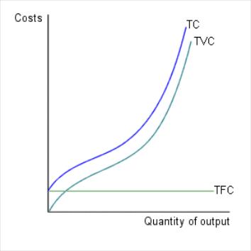
Notice that the variable and total cost curves are parallel, since the distance between them is a constant number – the fixed cost.