28. The effects of changes in income and prices

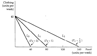
Income change (prices unchanged)	Price change (income unchanged)
Causes shifts of the budget line: – Right side if income became higher – Left side if income became lower	Causes turning of the budget line: – clockwise if the price of X-good decreased – counter-clockwise if the price increased

29 Equimarginal Principle and Consumer equilibrium

In order to maximize the utility derived from the two goods, the individual must allocate their budget to the “highest valued use.” This is accomplished by the use of marginal analysis. There are two steps to this process. First, the marginal utility of each unit of each good is considered. Second, the price of each good (or the relative prices) must be taken into account.

It is believed that as a person consumes more and more of a (homogeneous) good in a given period of time, that eventually the total utility (TU) derived from that good will increase at a decreasing rate; the point of diminishing marginal utility (MU) will be reached.

When there are two (or more) goods (with prices) and a budget, the individual will maximize TU by spending each additional dollar (euro, franc, pound or whatever monetary unit) on the good with the greatest marginal utility per unit of price MUx/Px.

This process may be referred to as the equimarginal principle. It is a useful tool and can be used to optimize (maximize or minimize) variables in marginal analysis. It will be used again to find the minimum cost per unit combination of inputs into a production process.

The rule for maximizing utility given a set of price and a budget is straightforward; if the marginal utility per dollar spent on good X is greater that the marginal utility per dollar spent of good Y, buy good X.

Utility is maximized when the marginal utility per dollar spent is the same for all goods. This can be expressed for as many goods as necessary. Since there is a budget constraint, if the marginal utility per dollar of one good is greater than the MU/$ of another and the budget is all spent, the individual should buy less of one to obtain more of the other. The equi-marginal principle can be expressed;

MUx/Px= MUy/Py=…= MUn/Pn

Consumer equilibrium occurs where the budget line is tangent to the highest attainable indifference curve. At this unique point, MRS = slope (price ratio of Px/Py)

30.Income Consumption Curve. Engel Curves

Holding the price of all goods constant, the income consumption curve for a good is the set of optimal bundles as income varies.

With the help of Income Consumption Curve we can plot Engel curve – the curve that shows the relationship between the quantity of a good consumed and income.

There are several configuration of Engel curve according to categories of goods it represents.

Inferior goods

31.Price Consumption Curve and Ind. Demand curve

H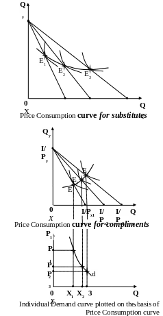 olding income and the prices of other goods constant, the price consumption curve for a good is the set of optimal bundles as the price of the good varies.

As we can see on the graphs the Price Consumption curve for compliments looks like the curve with positive slope which shows the direct relationship between consumption quantity of one good (X) and another good (Y). The opposite situation with the Price Consumption curve for substitutes: the relationship between consumption quantity of one good (X) and another good (Y) is inverse and the curve has negative slope. The individual demand curve takes a single good and explains the relationship between the cost of that good, and the quantity demanded. Therefore shifts in the indifference curves (PCC) based on consumption possibilities, should correlate to the shifts in the demand curves.