26. Indifference curves.

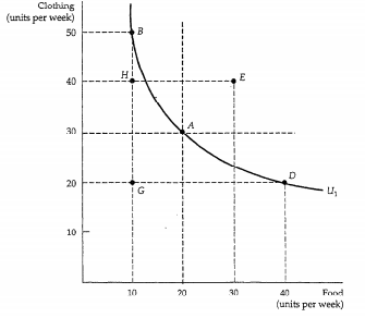
Indifferent curve is a curve showing the different combinations of two goods that provide the same satisfaction or total utility to a consumer.

Properties of Indifference Curves:

1. Every bundle is on some indifference curve;

2. Two indifference curves never cross;

3. Indifference curve slopes downward;

4. A bundle that has more of all goods is on a higher indifference curve.

A different level of satisfaction or total utility can be shown in indifference map - a selection of indifference curves.

One more characteristic of indifference curves is marginal rate of substitution (MRSxy). MRSxy is the rate at which a consumer is willing to substitute one good for another good without a change in total utility. The MRS equals the slope of an indifference curve at any point on the curve. It shows how much more of a good would a consumer require to compensate them for loss of a unit of another good. MRS measures willingness to make this substitution:

MRSxy= -ΔY/ΔX

On the graph we can see the way of MRS calculating.

The rate of MRS and therefore the form of indifferent curve depends on the relationships between examined goods.

For example, MRS for perfect substitutes is constant and hence the indifference curve looks like straight line (Picture (a)). And if goods are perfect complements MRS for them is zero, the indifference curves look like right angles(Picture (b)).

27.Budget ConstraintWhen goods are “free,” an individual should consume until the MU of a good is 0. This will insure that total utility is maximized. When goods are priced above zero and there is a finite budget, the utility derived from each expenditure must be maximized.

An individual will purchase a good when the utility derived from a unit of the good X (MUX) is greater than the utility derived from the money used to purchase the good (MU$). Let the price of a good (PX) represent the MU of money and the MUX represent the marginal benefit (MBX) of a purchase. When the PX > MBX, the individual should buy the good. If the PX < MBX, they should not buy the good. Where PX = MBX, they are in equilibrium, they should not change their purchases.

Given a finite budget (B) or income (I) and a set of prices of the goods (PX , PY, PN) that are to be purchased, a finite quantity of goods (QX, QY, QN) can be purchased. The budget constraint can be expressed,

B=PxQx + PyQy +…+ PnQn

Where B – budget, Pn – price of Nth good, Qn–quantity of Nth good

For one good the maximum amount that can be purchased is determined by the budget and the price of the good

Qx that can be perchased = Budget/Price=B/Px

The combinations of two goods that can be purchased can be shown graphically. The maximum of good X that can be purchased is B/ Px, the amount of the Y good is B/ Py. All possible combinations of good X and Y that can be purchased lie along (and inside) a line connecting the X and Y intercepts. This is shown in Figure.

The slope of the budget line equals the ratio of the price of good X on the horizontal axis divided by the price of good Y on the vertical axis.