1.Preferences, utility function, problem of choice, and the theory of demand. Preferences A decisionmaker always chooses its most preferred alternative from its set of available alternatives. So to model choice we must model decisionmakers’ preferences.

Preference Relations: Comparing two different consumption bundles, x and y:

strict preference: x is more preferred than is y.

weak preference: x is as at least as preferred as is y.

indifference: x is exactly as preferred as is y.

Strict preference, weak preference and indifference are all preference relations. Particularly, they are ordinal relations; i.e. they state only the order in which bundles are preferred.

denotes strict preference; x ≻ y means that bundle x is preferred strictly to bundle y.

~ denotes indifference; x ~ y means x and y are equally preferred.

≿ denotes weak preference; x ≿ y means x is preferred at least as much as is y.

Assumptions about Preference Relations:

Completeness: For any two bundles x and y it is always possible to make the statement that either x ≿ y or y ≿ x.

Reflexivity: Any bundle x is always at least as preferred as itself; i.e. x ≿ x.

Transitivity: If x is at least as preferred as y, and y is at least as preferred as z, then x is at least as preferred as z; i.e. x ≿ y and y ≿ z → x ≿ z.

Indifference CurvesTake: a reference bundle x’. The set of all bundles equally preferred to x’ is the indifference curve containing x’; the set of all bundles y ~ x’.Since an indifference “curve” is not always a curve a better name might be an indifference “set”.

Extreme Cases of Indifference Curves; Perfect Substitutes:If a consumer always regards units of commodities 1 and 2 as equivalent, then the commodities are perfect substitutes and only the total amount of the two commodities in bundles determines their preference rank-order.

Extreme Cases of Indifference Curves; Perfect Complements :If a consumer always consumes commodities 1 and 2 in fixed proportion (e.g. one-to-one), then the commodities are perfect complements and only the number of pairs of units of the two commodities determines the preference rank-order of bundles.

The slope of an indifference curve is its marginal rate-of-substitution (MRS). MRS at x’ is lim {Dx₂/Dx₁}= dx₂/dx₁ at x’

Utility Functions

A preference relation that is complete, reflexive, transitive and continuous can be represented by a continuous utility function.

Continuity means that small changes to a consumption bundle cause only small changes to the preference level.

A utility function U(x) represents a preference relation if and only if:

x’≻ x”↔ U(x’) > U(x”);x’ ≺x” ↔ U(x’) < U(x”); x’ ~ x”↔ U(x’) = U(x”).

Utility is an ordinal (i.e. ordering) concept. E.g. if U(x) = 6 and U(y) = 2 then bundle x is strictly preferred to bundle y. But x is not preferred three times as much as is y. Consider the bundles (4,1), (2,3) and (2,2). Suppose (2,3) (4,1) ~ (2,2). Assign to these bundles any numbers that preserve the preference ordering; e.g. U(2,3) = 6 > U(4,1) = U(2,2) = 4. Call these numbers utility levels.

An indifference curve contains equally preferred bundles. Equal preference Þ same utility level. Therefore, all bundles in an indifference curve have the same utility level. So the bundles (4,1) and (2,2) are in the indiff. curve with utility level U =4. But the bundle (2,3) is in the indiff. curve with utility level U= 6.

T he collection of all indifference curves for a given preference relation is an indifference map. An indifference map is equivalent to a utility function; each is the other. A good is a commodity unit which increases utility (gives a more preferred bundle). A bad is a commodity unit which decreases utility (gives a less preferred bundle). A neutral is a commodity unit which does not change utility (gives an equally preferred bundle). The marginal utility of commodity i is the rate-of-change of total utility as the quantity of commodity i consumed changes; i.e.

Marg. Rates-of-Substitution for Quasi-linear Utility Functions :MRS = - f (x₁) does not depend upon x₂ so the slope of indifference curves for a quasi-linear utility function is constant along any line for which x₁ is constant.

Choice. The principal behavioral postulate is that a decisionmaker chooses its most preferred alternative from those available to it. The available choices constitute the choice set.

The most preferred affordable bundle is called the consumer’s ORDINARY DEMAND at the given prices and budget. Ordinary demands will be denoted by x₁*(p₁,p₂,m) and x₂*(p₁,p₂,m).

Rational Constrained Choice:x₁*,x₂*) satisfies two conditions: (a) the budget is exhausted; p₁x₁* + p₂x₂* = m (b) the slope of the budget constraint, -p₁/p₂, and the slope of the indifference curve containing (x₁*,x₂*) are equal at (x₁*,x₂*).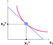

Demand. Comparative statics analysis of ordinary demand functions -- the study of how ordinary demands x₁*(p₁,p₂,y) and x₂*(p₁,p₂,y) change as prices p₁, p₂ and income y change. 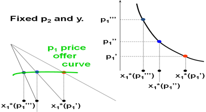The curve containing all the utility -maximizing bundles traced out as p₁ changes, with p₂ and y constant, is the p₁- price offer curve. The plot of the x₁-coordinate of the p₁- price offer curve against p₁ is the ordinary demand curve for commodity 1.

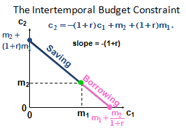
2. Intertemporal choice problem as foundation of the modern theory of finance.

Model of intertemporal choice involving consumption and investment decisions. (Named after Irving Fisher)

Irving Fisher developed the theory of Intertemporal Choice in 1930 in his book 'Theory of interest'. Contrary to Keynes, who related consumption to current income, Fisher’s model showed how rational forward looking consumers chooses consumption for the present and future to maximize their lifetime satisfaction. According to Fisher, an individual's impatience depends on four characteristics of his income stream: the size, the time shape, the composition and risk. Besides this foresight, self control, habit, expectation of life, and bequest motive (or concern for lives of others) are the five personal factors that determine a person's impatience which in turn determines his time preference. In order to understand the choice exercised by a consumer across different periods of time we take consumption in one period as a composite commodity. Suppose there is one consumer, N commodities, and two periods. Preferences are given by U (x1; x2) where xt = (xt1; :::; xtN ). Income in period t is Yt. Savings in period 1 is S1, spending in period t is Ct, and r is the interest rate.

C1 + S1 ≤Y1 ... (1)

C2 ≤ Y2 + S1 (1 + r) ... (2)

We arrive at the following equation from equation 1 and 2

= =

The left hand side shows the present value expenditure and right hand side depicts the present value income respectively. Multiplying the equation by (1+r) gives us the future value.

Now the consumer has to choose a C1 and C2 such that Max U(C1,C2) subject to C1+C2/(1+r) = Y1 + Y2/(1+r)

A consumer maybe a net saver or a net borrower. If he's initially at a level of consumption where he's neither of the above(i.e. a net borrower or net saver), an increase in income may make him a net saver or a net borrower depending on his preferences. An increase in current income or future income will increase current and future consumption(consumption smoothing motives).

Now, let us consider a scenario where the interest rates are increased. If the consumer is a net saver, he will save more in the current period due to the substitution effect and consume more in the current period due to the income effect. The net effect thus, becomes ambiguous. If the consumer is a net borrower, however, he will tend to consume less in the current period due to the substitution effect and income effect thereby reducing his overall current consumption.

If the consumer is a net saver, an increase in interest rate will have an ambiguous effect on the current consumption.

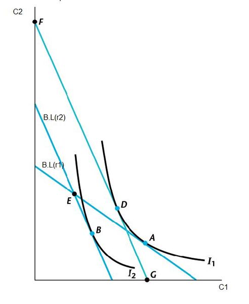
If the consumer is a net borrower, an increase in interest rate will reduce his current consumption.

Key Assumptions:

• Two periods (generalizing to many future periods is straightforward); Perfect capital markets; the absence of uncertainty

What is the consumer choosing? One of the many possible “Consumption Streams”. A consumption stream is a sequence of time dated consumption. Consumers are able to choose between alternative consumption streams. Choices are consistent (transitive), they prefer more consumption to less, i.e. they prefer higher standards of living to lower. Consumers choose the most preferred consumption stream among those attainable. Let m₁ and m₂ be incomes received in periods 1 and 2. Let c₁ and c₂ be consumptions in periods 1 and 2. Let p₁ and p₂ be the prices of consumption in periods 1 and 2. Suppose prices are 1$. Suppose that the consumer chooses not to save or to borrow. What will be consumed in period 1? c₁ = m₁. What will be consumed in period 2? c₂ = m₂.

Now suppose that the consumer spends nothing on consumption in period 1; that is, c₁ = 0 and the consumer saves s₁ = m₁. The interest rate is r. What now will be period 2’s consumption level?

Now suppose that the consumer spends everything possible on consumption in period 1, so c₂ = 0. What is the most that the consumer can borrow in period 1 against her period 2 income of $m₂? Let b₁ denote the amount borrowed in period 1. Only $m₂ will be available in period 2 to pay back $b₁ borrowed in period 1. So b₁(1 + r ) = m₂. That is, b₁ = m₂ / (1 + r ). So the largest possible period 1 consumption level is .

The calculation of saving or borrowing amounts is the modern theory of finance. All these calculation used in calculation of investing or spending cash flows. For example, bond, securities etc.