Introduction to convolutional codes

When we studied linear block codes, we described them in three ways:

1. The generator matrix describes how to turn a string of K arbitrary source bits into a transmission of N bits.

2. The parity-check matrix specifies the M = N – K parity-check constraints that a valid codeword satisfies.

3. The trellis of the code describes its valid codewords in terms of paths through a trellis with labelled edges.

We will now describe convolutional codes in two ways: first, in terms of mechanisms for generating transmissions t from source bits s; and second, in terms of trellises that describe the constraints satisfied by valid transmissions.

Linear-feedback shift-registers

We generate a transmission with a convolutional code by putting a source stream through a linear filter. This filter makes use of a shift register, linear output functions, and, possibly, linear feedback.

We will draw the shift-register in a right-to-left orientation: bits roll from right to left as time goes on.

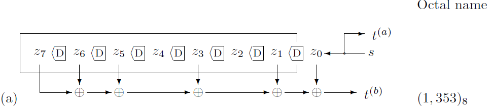
Figures show three linear-feedback shift-registers which could be used to define convolutional codes. The rectangular box surrounding the bits z₁ … z₇ indicates the memory of the filter, also known as its state. The filters are (a) systematic and non-recursive; (b) non-systematic and non-recursive; (c) systematic and recursive. All three filters have one input and two outputs. On each clock cycle, the source supplies one bit, and the filter outputs two bits t^(a) and t^(b). By concatenating together these bits we can obtain from our source stream s₁s₂s₃ … a transmission stream Because there are two transmitted bits for every source bit, the codes shown in figures have rate 1/2. Because these filters require k = 7 bits of memory, the codes they define are known as a constraint-length 7 codes.

Convolutional codes come in three flavours, corresponding to the three types of filter.

Systematic non-recursive

The filter shown in figure a has no feedback. It also has the property that one of the output bits, t^(a), is identical to the source bit s. This encoder is thus called systematic, because the source bits are reproduced transparently in the transmitted stream, and non-recursive, because it has no feedback. The other transmitted bit t^(b) is a linear function of the state of the filter. One way of describing that function is as a dot product (modulo 2) between two binary vectors of length k + 1: a binary vector g^(b) = (1, 1, 1, 0, 1, 0, 1, 1) and the state vector z = (z_k; z_k-1, … , z₁; z₀). We include in the state vector the bit z₀ that will be put into the first bit of the memory on the next cycle. The vector g^(b) has g_τ^(b) = 1 for every τ where there is a tap (a downward pointing arrow) from state bit z_τ into the transmitted bit t^(b).

A convenient way to describe these binary tap vectors is in octal. Thus, this filter makes use of the tap vector 353₈.

11 101 011

↓ ↓ ↓

3 5 3

Nonsystematic nonrecursive

The filter shown in figure b also has no feedback, but it is not systematic. It makes use of two tap vectors g^(a) and g^(b) to create its two transmitted bits. This encoder is thus nonsystematic and nonrecursive. Because of their added complexity, nonsystematic codes can have error-correcting abilities superior to those of systematic nonrecursive codes with the same constraint length.

Systematic recursive

The filter shown in figure c is similar to the nonsystematic nonrecursive filter shown in figure b, but it uses the taps that formerly made up g^(a) to make a linear signal that is fed back into the shift register along with the source bit. The output t^(b) is a linear function of the state vector as before. The other output is t^(a) = s, so this filter is systematic.

A recursive code is conventionally identified by an octal ratio, e.g., figure c's code is denoted by (247/371)₈.

Joint entropy

Often we are interested in the entropy of pairs of random variables (X, Y ). Another way of thinking of this is as a vector of random variables.

Definition 1 If X and Y are jointly distributed according to p(X, Y), then the joint entropy H(X, Y) is

or

#

Definition 2 If , then the conditional entropy is

or

#

Theorem 1 (chain rule)

Interpretation: The uncertainty (entropy) about both X and Y is equal to the uncertainty (entropy) we have about X, plus whatever we have about Y , given that we know X.

Proof This proof is very typical of the proofs in this class: it consists of a long string of equalities. (Later proofs will consist of long strings of inequalities. Some people make their livelihood out of inequalities!)

#

We can also have a joint entropy with a conditioning on it, as shown in the following corollary:

Corollary 1

The proof is similar to the one above.

Jointly-typical sequences

Formalization of the intuitive preview.

We will define codewords x^(s) as coming from an ensemble X^N, and consider the random selection of one codeword and a corresponding channel output y, thus defining a joint ensemble (XY)^N. We will use a typical-set decoder, which decodes a received signal y as s if x^(s) and y are jointly typical, a term to be defined shortly.

The proof will then centre on determining the probabilities (a) that the true input codeword is not jointly typical with the output sequence; and (b) that a false input codeword is jointly typical with the output. We will show that, for large N, both probabilities go to zero as long as there are fewer than 2^NC codewords, and the ensemble X is the optimal input distribution.

Joint typicality theorem. Let x, y be drawn from the ensemble (XY)^N defined by

Then

1. the probability that x, y are jointly typical (to tolerance β) tends to 1 as N → ∞;

2. the number of jointly-typical sequences |J_Nβ| is close to 2^NH(X;Y). To be precise,

3. if x` ~ X<sup>N</sup> and y` ~ Y^N, i.e., x` and y` are independent samples with the same marginal distribution as P(x, y), then the probability that (x`, y`) lands in the jointly-typical set is about 2^–NI(X;Y). To be precise,

Random coding and typical-set decoding

Consider the following encoding-decoding system, whose rate is R`.

1. We fix P(x) and generate the S = 2<sup>NR`</sup> codewords of a (N,NR`) = (N,K) code C at random according to

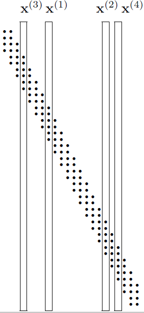
Figure A random code.

2. The code is known to both sender and receiver.

3. A message s is chosen from {1, 2, . . . , 2^NR`}, and x^(s) is transmitted. The received signal is y, with

4. The signal is decoded by typical-set decoding. Typical-set decoding. Decode y as ŝ if (x^(ŝ), y) are jointly typical and there is no other s` such that (x<sup>(s`)</sup>, y) are jointly typical; otherwise declare a failure (ŝ =0).

This is not the optimal decoding algorithm, but it will be good enough, and easier to analyze.

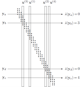
Figure example decodings by the typical set decoder. A sequence that is not jointly typical with any of the codewords, such as y_a, is decoded as ŝ = 0. A sequence that is jointly typical with codeword x⁽³⁾ alone, y_b, is decoded as ŝ = 3. Similarly, y_c is decoded as ŝ = 4. A sequence that is jointly typical with more than one codeword, such as y_d, is decoded as ŝ = 0.

K-means clustering

About the name… the `K' in K-means clustering simply refers to the chosen number of clusters. If Newton had followed the same naming policy, maybe we would learn at school about ‘calculus for the variable x’. It's a silly name, but we are stuck with it.

The K-means algorithm is an algorithm for putting N data points in an I-dimensional space into K clusters. Each cluster is parameterized by a vector m^(k) called its mean.

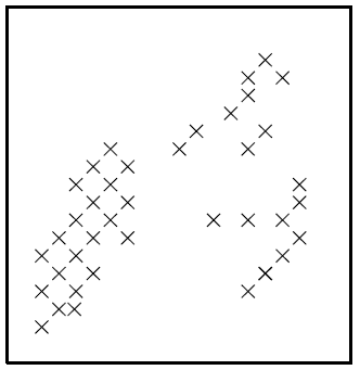
Figure. N = 40 data points.

The data points will be denoted by {x⁽ⁿ⁾} where the superscript n runs from 1 to the number of data points N. Each vector x has I components x_i. We will assume that the space that x lives in is a real space and that we have a metric that defines distances between points, for example,

To start the K-means algorithm, the K means {m^(k)} are initialized in some way, for example to random values. K-means is then an iterative two-step algorithm. In the assignment step, each data point n is assigned to the nearest mean. In the update step, the means are adjusted to match the sample means of the data points that they are responsible for.

Algorithm. The K-means clustering algorithm.

Initialization. Set K means {m^(k)} to random values.

Assignment step. Each data point n is assigned to the nearest mean. We denote our guess for the cluster k⁽ⁿ⁾ that the point x⁽ⁿ⁾ belongs to by .

An alternative, equivalent representation of this assignment of points to clusters is given by ‘responsibilities’, which are indicator variables r_k⁽ⁿ⁾. In the assignment step, we set r_k⁽ⁿ⁾ to one if mean k is the closest mean to datapoint x⁽ⁿ⁾; otherwise r_k⁽ⁿ⁾ is zero.

What about ties? – We don't expect two means to be exactly the same distance from a data point, but if a tie does happen, is set to the smallest of the winning {k}.

Update step. The model parameters, the means, are adjusted to match the sample means of the data points that they are responsible for.

where R^(k) is the total responsibility of mean k,

What about means with no responsibilities? – If R^(k)= 0, then we leave the mean m^(k) where it is.

The K-means algorithm with a larger number of means, 4, is demonstrated. The outcome of the algorithm depends on the initial condition.

In the first case, after five iterations, a steady state is found in which the data points are fairly evenly split between the four clusters. In the second case, after six iterations, half the data points are in one cluster, and the others are shared among the other three clusters.

A final criticism of K-means is that it is a ‘hard’ rather than a ‘soft’ algorithm: points are assigned to exactly one cluster and all points assigned to a cluster are equals in that cluster. Points located near the border between two or more clusters should, arguably, play a partial role in determining the locations of all the clusters that they could plausibly be assigned to. But in the K-means algorithm, each borderline point is dumped in one cluster, and has an equal vote with all the other points in that cluster, and no vote in any other clusters.

Lempel–Ziv coding

The Lempel-Ziv algorithms, which are widely used for data compression (e.g., the compress and gzip commands), are different in philosophy to arithmetic coding. There is no separation between modelling and coding, and no opportunity for explicit modelling.

Basic Lempel-Ziv algorithm

The method of compression is to replace a substring with a pointer to an earlier occurrence of the same substring. For example if the string is 1011010100010. . . , we parse it into an ordered dictionary of substrings that have not appeared before as follows: λ, 1, 0, 11, 01, 010, 00, 10, . . . . We include the empty substring λ as the first substring in the dictionary and order the substrings in the dictionary by the order in which they emerged from the source. After every comma, we look along the next part of the input sequence until we have read a substring that has not been marked off before. A moment's reflection will confirm that this substring is longer by one bit than a substring that has occurred earlier in the dictionary. This means that we can encode each substring by giving a pointer to the earlier occurrence of that prefix and then sending the extra bit by which the new substring in the dictionary differs from the earlier substring. If, at the n^th bit, we have enumerated s(n) substrings, then we can give the value of the pointer in bits. The code for the above sequence is then as shown in the fourth line of the following table (with punctuation included for clarity), the upper lines indicating the source string and the value of s(n):

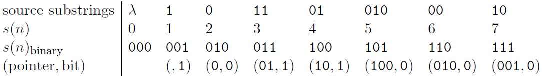
Notice that the first pointer we send is empty, because, given that there is only one substring in the dictionary – the string λ – no bits are needed to convey the “choice” of that substring as the prefix. The encoded string is 100011101100001000010. The encoding, in this simple case, is actually a longer string than the source string, because there was no obvious redundancy in the source string.

One reason why the algorithm described above lengthens a lot of strings is because it is inefficient – it transmits unnecessary bits; to put it another way, its code is not complete. Once a substring in the dictionary has been joined there by both of its children, then we can be sure that it will not be needed (except possibly as part of our protocol for terminating a message); so at that point we could drop it from our dictionary of substrings and shuffle them all along one, thereby reducing the length of subsequent pointer messages. Equivalently, we could write the second prefix into the dictionary at the point previously occupied by the parent. A second unnecessary overhead is the transmission of the new bit in these cases – the second time a prefix is used, we can be sure of the identity of the next bit.

Decoding

The decoder again involves an identical twin at the decoding end who constructs the dictionary of substrings as the data are decoded.

Example Encode the string 000000000000100000000000 using the basic Lempel-Ziv algorithm described above.

The encoding is 010100110010110001100, which comes from the parsing

0, 00, 000, 0000, 001, 00000, 000000

which is encoded thus:

(, 0), (1, 0), (10, 0), (11, 0), (010, 1), (100, 0), (110, 0)

Decode the string 00101011101100100100011010101000011 that was encoded using the basic Lempel-Ziv algorithm.

The decoding is 0100001000100010101000001

Low-Density Parity-Check Codes

A low-density parity-check code (or Gallager code) is a block code that has a parity-check matrix, H, every row and column of which is ‘sparse’.

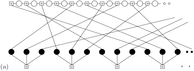
A regular Gallager code is a low-density parity-check code in which every column of H has the same weight j and every row has the same weight k; regular Gallager codes are constructed at random subject to these constraints. A low-density parity-check code with j = 3 and k = 4 is illustrated in figure

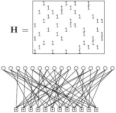
A low-density parity-check matrix and the corresponding graph of a rate-1/4 low-density parity-check code with blocklength N = 16, and M = 12 constraints. Each white circle represents a transmitted bit. Each bit participates in j = 3 constraints, represented by squares. Each constraint forces the sum of the k = 4 bits to which it is connected to be even.

Theoretical properties

Low-density parity-check codes, in spite of their simple construction, are good codes, given an optimal decoder. These result hold for any column weight j ≥ 3.

However, we don't have an optimal decoder, and decoding low-density parity-check codes is an NP-complete problem. So what can we do in practice?

Practical decoding

Given a channel output r, we wish to find the codeword t whose likelihood P(r | t) is biggest. All the effective decoding strategies for low-density paritycheck codes are message-passing algorithms. The best algorithm known is the sum–product algorithm, also known as iterative probabilistic decoding or belief propagation.

We'll assume that the channel is a memoryless channel (though more complex channels can easily be handled by running the sum–product algorithm on a more complex graph that represents the expected correlations among the errors). For any memoryless channel, there are two approaches to the decoding problem, both of which lead to the generic problem – find the x that maximizes

where P(x) is a separable distribution on a binary vector x, and z is another binary vector. Each of these two approaches represents the decoding problem in terms of a factor graph.

Maximum Likelihood and Clustering

Rather than enumerate all hypotheses – which may be exponential in number – we can save a lot of time by homing in on one good hypothesis that fits the data well. This is the philosophy behind the maximum likelihood method, which identifies the setting of the parameter vector θ that maximizes the likelihood, P(Data | θ,H).

For some models the maximum likelihood parameters can be identified instantly from the data; for more complex models, finding the maximum likelihood parameters may require an iterative algorithm.

For any model, it is usually easiest to work with the logarithm of the likelihood rather than the likelihood, since likelihoods, being products of the probabilities of many data points, tend to be very small. Likelihoods multiply; log likelihoods add.

Maximum likelihood for a mixture of Gaussians

We now derive an algorithm for fitting a mixture of Gaussians to one-dimensional data. In fact, this algorithm is so important to understand that, we, get to derive the algorithm.

Problem. A random variable x is assumed to have a probability distribution that is a mixture of two Gaussians,

where the two Gaussians are given the labels k = 1 and k = 2; the prior probability of the class label k is {p₁ =1/2; p₂=1/2}; {μ_k} are the means of the two Gaussians; and both have standard deviation σ. For brevity, we denote these parameters by θ≡{{μ_k}, σ }.

A data set consists of N points {x_n}^N_n=1 which are assumed to be independent samples from this distribution. Let k_n denote the unknown class label of the nth point.

Assuming that {μ_k} and σ are known, show that the posterior probability of the class label k_n of the nth point can be written as

and give expressions for w₁ and w₀.

Maximum likelihood for one Gaussian

We return to the Gaussian for our first examples. Assume we have data {x_n}^N_n=1. The log likelihood is:

The likelihood can be expressed in terms of two functions of the data, the sample mean

and the sum of square deviations

Because the likelihood depends on the data only through and S, these two quantities are known as sufficient statistics.

Example. Differentiate the log likelihood with respect to μ and show that, if the standard deviation is known to be σ, the maximum likelihood mean μ of a Gaussian is equal to the sample mean , for any value of σ.

Solution.

If we Taylor-expand the log likelihood about the maximum, we can define approximate error bars on the maximum likelihood parameter: we use a quadratic approximation to estimate how far from the maximum-likelihood parameter setting we can go before the likelihood falls by some standard factor, for example e^1/2, or e^4/2. In the special case of a likelihood that is a Gaussian function of the parameters, the quadratic approximation is exact.

Message classification

Time

• continuous – stochastic time function;

• discrete – chain of stochastic events.

Set

• continuous – function may possess the range of values in an interval;

• discrete – may possess a finite set of discrete values.

Message classifications:

а) continuous in set and time

б) continuous in set, discrete in time

в) discrete in set, continuous in time

г) discrete in set and time

Message Passing

It turns out that quite a few interesting problems can be solved by message-passing algorithms, in which simple messages are passed locally among simple processors whose operations lead, after some time, to the solution of a global problem.

Counting

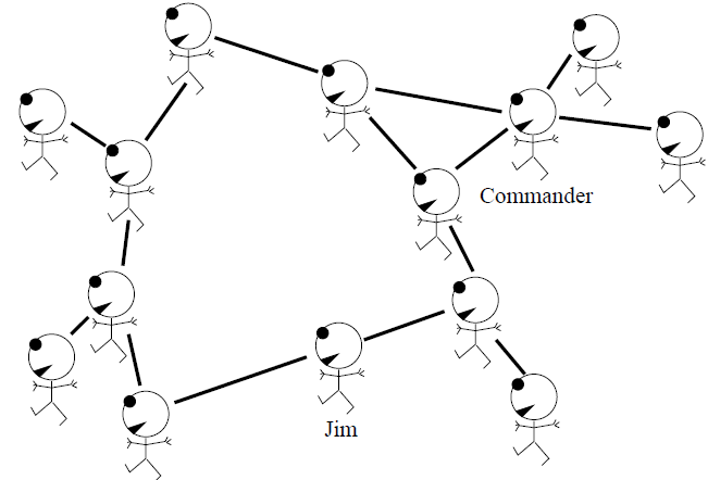
As an example, consider a line of soldiers walking in the mist. The commander wishes to perform the complex calculation of counting the number of soldiers in the line. This problem could be solved in two ways.

First there is a solution that uses expensive hardware: the loud booming voices of the commander and his men. The commander could shout “all soldiers report back to me within one minute!”, then he could listen carefully as the men respond ‘Molesworth here sir!”, “Fotherington-Thomas here sir!”, and so on. This solution relies on several expensive pieces of hardware: there must be a reliable communication channel to and from every soldier; the commander must be able to listen to all the incoming messages – even when there are hundreds of soldiers – and must be able to count; and all the soldiers must be well-fed if they are to be able to shout back across the possibly-large distance separating them from the commander.

The second way of finding this global function, the number of soldiers, does not require global communication hardware, high IQ, or good food; we simply require that each soldier can communicate single integers with the two adjacent soldiers in the line, and that the soldiers are capable of adding one to a number.

This solution requires only local communication hardware and simple computations (storage and addition of integers).

Separation

This clever trick makes use of a profound property of the total number of soldiers: that it can be written as the sum of the number of soldiers in front of a point and the number behind that point, two quantities which can be computed separately, because the two groups are separated by the commander.

If the soldiers were not arranged in a line but were travelling in a swarm, then it would not be easy to separate them into two groups in this way.

More on trellises

We now discuss various ways of making the trellis of a code.

The span of a codeword is the set of bits contained between the first bit in the codeword that is non-zero, and the last bit that is non-zero, inclusive. We can indicate the span of a codeword by a binary vector as shown in table

A generator matrix is in trellis-oriented form if the spans of the rows of the generator matrix all start in different columns and the spans all end in different columns.

How to make a trellis from a generator matrix

First, put the generator matrix into trellis-oriented form by row-manipulations similar to Gaussian elimination. For example, our (7; 4) Hamming code can be generated by

but this matrix is not in trellis-oriented form – for example, rows 1, 3 and 4 all have spans that end in the same column. By subtracting lower rows from upper rows, we can obtain an equivalent generator matrix (that is, one that generates the same set of codewords) as follows:

Trellises from parity-check matrices

Another way of viewing the trellis is in terms of the syndrome. The syndrome of a vector r is defined to be Hr, where H is the parity-check matrix. A vector is only a codeword if its syndrome is zero. As we generate a codeword we can describe the current state by the partial syndrome, that is, the product of H with the codeword bits thus far generated. Each state in the trellis is a partial syndrome at one time coordinate. The starting and ending states are both constrained to be the zero syndrome. Each node in a state represents a different possible value for the partial syndrome. Since H is an M×N matrix, where M = N – K, the syndrome is at most an M-bit vector. So we need at most 2^M nodes in each state. We can construct the trellis of a code from its parity-check matrix by walking from each end, generating two trees of possible syndrome sequences. The intersection of these two trees defines the trellis of the code.

More than two variables

It will be important to deal with more than one or two variables, and a variety of “chain rules” have been developed for this purpose. In each of these, the sequence of r.v.s are drawn according to the joint distribution .

Theorem 3 The joint entropy of is

Proof Observe that

An alternate proof can be obtained by observing that

and taking an expectation.

#

We sometimes have two variables that we wish to consider, both conditioned upon another variable.

Definition 5 The conditional mutual information of random variables X and Y given Z is defined by

In other words, it is the same as mutual information, but everything is conditioned upon Z. The chain rule for entropy leads us to a chain rule for mutual information.

Theorem 4

Proof

Noise and distortion in the channels of information transmission.

Noisy channels

A discrete memoryless channel Q is characterized by an input alphabet χ_X, an output alphabet χ_Y , and a set of conditional probability distributions P(y | x), one for each x.

These transition probabilities may be written in a matrix

Q_j|i = P(y=b_j | x=a_i)

This matrix has the output variable j indexing the rows and the input variable i indexing the columns, so that each column of Q is a probability vector. With this convention, we can obtain the probability of the output, p_Y , from a probability distribution over the input, p_X, by right-multiplication:

p_Y = Qp_X

Some useful model channels are:

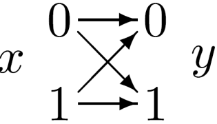
Binary symmetric channel. χ_X ={0, 1}. χ_Y ={0, 1}.

P(y=0 | x=0) = 1 – f;

P(y=1 | x=0) = f;

P(y=0 | x=1) = f;

P(y=1 | x=1) = 1 – f.

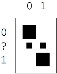
Binary erasure channel. χ_X ={0, 1}. χ_Y ={0, ?, 1}.

P(y=0 | x=0) = 1 – f;

P(y=? | x=0) = f;

P(y=1 | x=0) = 0;

P(y=0 | x=1) = 0;

P(y=? | x=1) = f;

P(y=1 | x=1) = 1 – f.

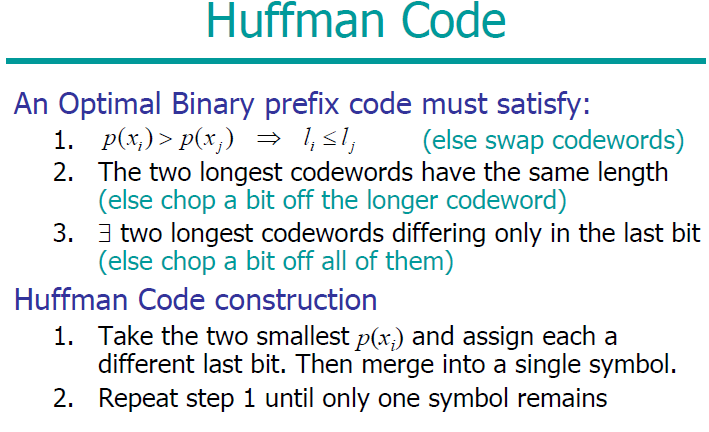
Optimal source coding with symbol codes: Huffman coding

1. Take the two least probable symbols in the alphabet. These two symbols will be given the longest codewords, which will have equal length, and differ only in the last digit.

2. Combine these two symbols into a single symbol, and repeat. Since each step reduces the size of the alphabet by one, this algorithm will have assigned strings to all the symbols after | χ^X| – 1 steps.

Example Let χ^X ={a, b, c, d, e}

and P_X ={0.25, 0.25, 0.2, 0.15, 0.15}.

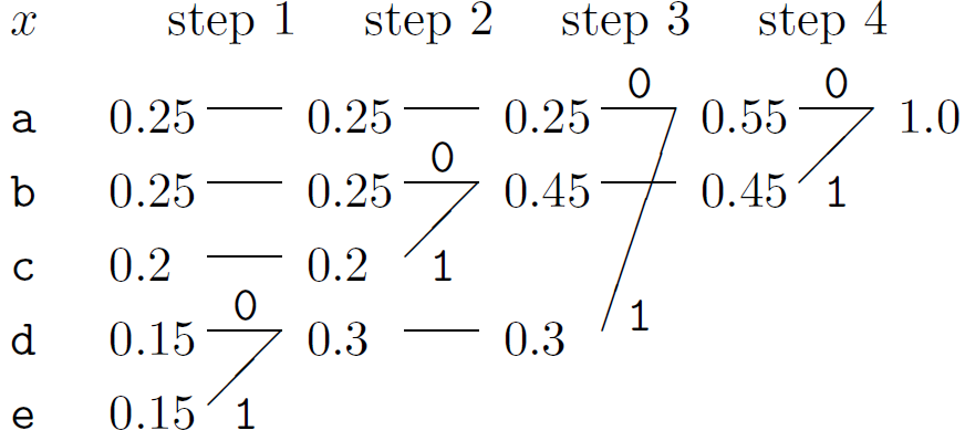
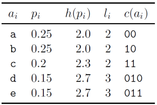
The codewords are then obtained by concatenating the binary digits in reverse order: C = {00, 10, 11, 010, 011}. The codelengths selected by the Huffman algorithm (column 4) are in some cases longer and in some cases shorter than the ideal codelengths, the Shannon information contents log₂1/pi (column 3). The expected length of the code is L = 2.30 bits, whereas the entropy is H = 2.2855 bits.

If at any point there is more than one way of selecting the two least probable symbols then the choice may be made in any manner – the expected length of the code will not depend on the choice.

Other roles for hash codes

Checking arithmetic

If you wish to check an addition that was done by hand, you may find useful the method of casting out nines. In casting out nines, one finds the sum, modulo nine, of all the digits of the numbers to be summed and compares it with the sum, modulo nine, of the digits of the putative answer. [With a little practice, these sums can be computed much more rapidly than the full original addition.]

Example

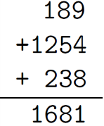
The sum, modulo nine, of the digits in 189+1254+238 is 7, and the sum, modulo nine, of 1+6+8+1 is 7. The calculation thus passes the casting-out-nines test.

Casting out nines gives a simple example of a hash function. For any addition expression of the form a + b + c + …, where a, b, c, … are decimal numbers we define h from {0, 1, 2, 3, 4, 5, 6, 7, 8} by

h(a + b + c + …) = sum modulo nine of all digits in a, b, c

then it is nice property of decimal arithmetic that if a + b + c + … = m + n + o + …

then the hashes h(a + b + c + …) and h(m + n + o + …) are equal.

Error detection among files

Are two files the same? If the files are on the same computer, we could just compare them bit by bit. But if the two files are on separate machines, it would be nice to have a way of confirming that two files are identical without having to transfer one of the files from A to B. [And even if we did transfer one of the files, we would still like a way to confirm whether it has been received without modifications!]

Tamper detection

What if the differences between the two files are not simply `noise', but are introduced by an adversary, a clever forger called Fiona, who modifies the original file to make a forgery that purports to be Alice's file? How can Alice make a digital signature for the file so that Bob can confirm that no-one has tampered with the file? And how can we prevent Fiona from listening in on Alice's signature and attaching it to other files?

Let's assume that Alice computes a hash function for the file and sends it securely to Bob. If Alice computes a simple hash function for the file like the linear cyclic redundancy check, and Fiona knows that this is the method of verifying the file's integrity, Fiona can make her chosen modifications to the file and then easily identify (by linear algebra) a further 32-or-so single bits that, when flipped, restore the hash function of the file to its original value.

Parity-check matrices of convolutional codes and turbo codes

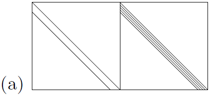
Figure. Schematic pictures of the parity-check matrices of (a) a convolutional code, rate 1/2, and (b) a turbo code, rate 1/3. Notation: A diagonal line represents an identity matrix. A band of diagonal lines represent a band of diagonal 1s. A circle inside a square represents the random permutation of all the columns in that square. A number inside a square represents the number of random permutation matrices superposed in that square. Horizontal and vertical lines indicate the boundaries of the blocks within the matrix.

We close by discussing the parity-check matrix of a rate-1/2 convolutional code viewed as a linear block code. We adopt the convention that the N bits of one block are made up of the N=2 bits t^(a) followed by the N=2 bits t^(b).

The parity-check matrix of a turbo code can be written down by listing the constraints satisfied by the two constituent trellises (figure b). So turbo codes are also special cases of low-density parity-check codes. If a turbo code is punctured, it no longer necessarily has a low-density parity-check matrix, but it always has a generalized parity-check matrix that is sparse.

Periods of information circulation

IS has following stages of information flow:

1. Information perception stage

2. Information preparation stage

3. Information transmission and storage stage

4. Information process stage

5. Information representation stage

6. Influence stage

1. On the information perception stage an actor extracts and analyses information about the object of observation and control. As a result it creates an image of that object and produces its recognition and evaluation.

2. On the information preparation stage an actor normalizes received information and produces analog-digital conversion and coding of information. This stage could be considered as subsidiary on the stage of information perception. As a result of information perception and preparation will be created a signal which could be transmitted and/or processed.

3. On the stage of information transmission and storage – information is being transmitted form source to destination (in space and time). Mechanisms and problems of information transmission and storage are very coherent to each other. For that purposes different physical environment could be used (electric, electro-magnetic, optic, etc.).

4. On the stage of information process general interferences valuable for system could be emphasized. Transformation of information could be realized by an actor (human being, computer, etc.). Different actors have different abilities to process information. E.g. if this process could be formalized and abstracted it could be done automatically on computer; if this process requires creativity - nobody but human may handle it. For example, the main aim of information process in control systems is making decision regarding choice of control instruments.

5. Stage of information representation is very important in processes when human operator involved. The aim of this stage is to provide operator with all necessary information regarding system using IO devices.

6. On the stage of influence – information being used for performance of required changes in system. Signals produces regulative or control actions creating changes inside the object of control.

Pictorial demonstration of Gallager codes

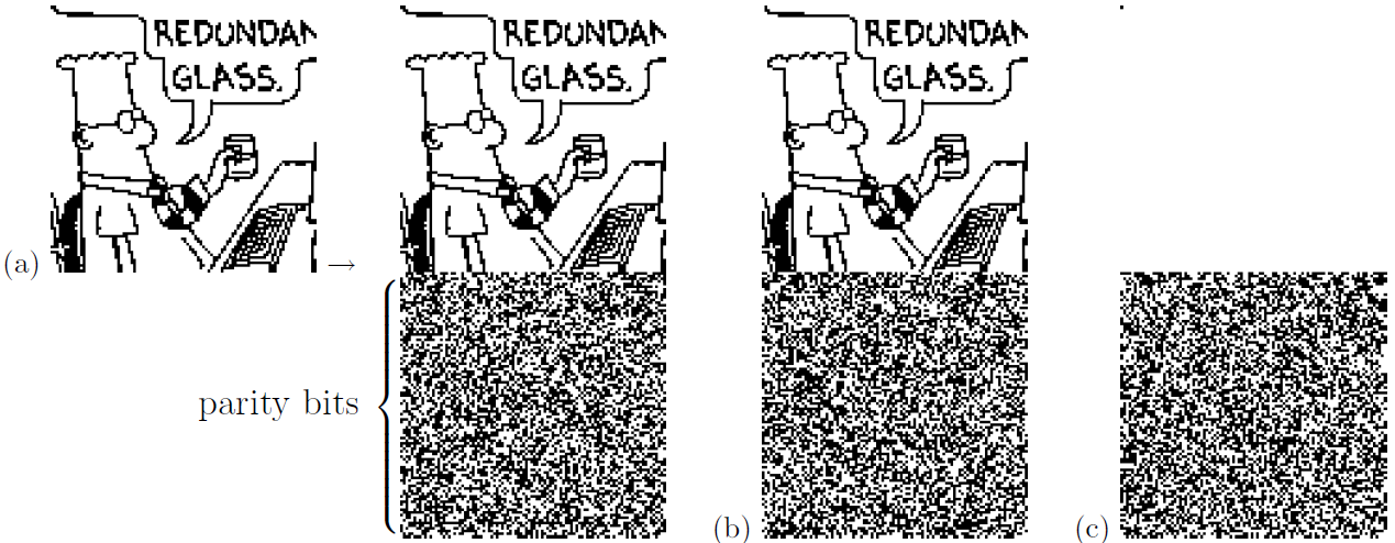
Figure demonstrate encoding with a rate -1/2 Gallager code. The encoder is derived from a very sparse 10 000 × 20 000 parity-check matrix with three 1s per column. (a) The code creates transmitted vectors consisting of 10 000 source bits and 10 000 paritycheck bits. (b) Here, the source sequence has been altered by changing the first bit. Notice that many of the parity-check bits are changed. Each parity bit depends on about half of the source bits. (c) The transmission for the case s = (1, 0, 0, …, 0). This vector is the difference (modulo 2) between transmissions (a) and (b).

Encoding

Figure illustrates the encoding operation for the case of a Gallager code whose parity-check matrix is a 10 000 × 20 000 matrix with three 1s per column. The high density of the generator matrix is illustrated in figure b and c by showing the change in the transmitted vector when one of the 10 000 source bits is altered. Of course, the source images shown here are highly redundant, and such images should really be compressed before encoding. Redundant images are chosen in these demonstrations to make it easier to see the correction process during the iterative decoding. The decoding algorithm does not take advantage of the redundancy of the source vector, and it would work in exactly the same way irrespective of the choice of source vector.

Iterative decoding

The transmission is sent over a channel with noise level f = 7.5% and the received vector is shown in the upper left of figure. The subsequent pictures in figure show the iterative probabilistic decoding process. The sequence of figures shows the best guess, bit by bit, given by the iterative decoder, after 0, 1, 2, 3, 10, 11, 12, and 13 iterations. The decoder halts after the 13th iteration when the best guess violates no parity checks. This final decoding is error free.

In the case of an unusually noisy transmission, the decoding algorithm fails to find a valid decoding. For this code and a channel with f = 7.5%, such failures happen about once in every 100 000 transmissions.

Planning for collisions

Example (Birthday problem) Given twenty-four people in a room, what is the probability that there are at least two people present who have the same birthday (i.e., day and month of birth)? What is the expected number of pairs of people with the same birthday? Which of these two questions is easiest to solve? Which answer gives most insight? A = number of days in year = 365 and S = number of people = 24.

Solution. The probability that S = 24 people whose birthdays are drawn at random from A = 365 days all have distinct birthdays is

The probability that two (or more) people share a birthday is one minus this quantity, which, for S = 24 and A = 365, is about 0.5. This exact way of answering the question is not very informative since it is not clear for what value of S the probability changes from being close to 0 to being close to 1.

The number of pairs is S(S – 1)/2, and the probability that a particular pair shares a birthday is 1/A, so the expected number of collisions is

This answer is more instructive. The expected number of collisions is tiny if and big if .

We can also approximate the probability that all birthdays are distinct, for small S, thus:

Probabilities and Inference

The number of inference problems that can (and perhaps should) be tackled by Bayesian inference methods is enormous. In this course, for example, we discuss the decoding problem for error-correcting codes, the task of inferring clusters from data, the task of interpolation through noisy data, and the task of classifying patterns given labelled examples. Most techniques for solving these problems can be categorized as follows.

Exact methods compute the required quantities directly. Only a few interesting problems have a direct solution, but exact methods are important as tools for solving subtasks within larger problems.

Approximate methods can be subdivided into

1. Deterministic approximations, which include maximum likelihood, Laplace's method and variational methods ; and

2. Monte Carlo methods – techniques in which random numbers play an integral part.

A widespread misconception is that the aim of inference is to find the most probable explanation for some data. While this most probable hypothesis may be of interest, and some inference methods do locate it, this hypothesis is just the peak of a probability distribution, and it is the whole distribution that is of interest. As we saw before, the most probable outcome from a source is often not a typical outcome from that source. Similarly, the most probable hypothesis given some data may be atypical of the whole set of reasonablyplausible hypotheses.

Relative entropy and mutual information

Suppose there is a r.v. with true distribution p. Then (as we will see) we could represent that r.v. with a code that has average length H(p). However, due to incomplete information we do not know p; instead we assume that the distribution of the r.v. is q. Then (as we will see) the code would need more bits to represent the r.v. The difference in the number of bits is denoted as . The quantity comes up often enough that it has a name: it is known as the relative entropy.

Definition 3 The relative entropy or Kullback-Leibler distance between two probability mass functions p(x) and q(x) is defined as

Note that this is not symmetric, and the q (the second argument) appears only in the denominator.

Another important concept is that of mutual information. How much information does one random variable tell about another one. In fact, this perhaps the central idea in much of information theory. When we look at the output of a channel, we see the outcomes of a r.v. What we want to know is what went into the channel – we want to know what was sent, and the only thing we have is what came out. The channel coding theorem (which is one of the high points we are trying to reach in the class) is basically a statement about mutual information.

Definition 4 Let X and Y be r.v.s with joint distribution p(X,Y) and marginal distributions p(x) and p(y). The mutual information I(X;Y) is the relative entropy between the joint distribution and the product distribution:

#

Note that when X and Y are independent, p(x,y) = p(x)p(y) (definition of independence), so I(X; Y) = 0. This makes sense: if they are independent random variables then Y can tell us nothing about X.

An important interpretation of mutual information comes from the following.

Theorem 2

Interpretation: The information that Y tells us about X is the reduction in uncertainty about X due to the knowledge of Y .

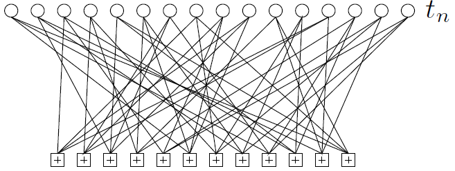
Repeat–Accumulate Codes

Repeat–accumulate codes were studied by Divsalar et al. (1998) for theoretical purposes, as simple turbo-like codes that might be more amenable to analysis than messy turbo codes. Their practical performance turned out to be just as good as other sparse-graph codes

The encoder

1. Take K source bits.

s₁s₂s₃ … s_K

2. Repeat each bit three times, giving N = 3K bits.

s₁s₁s₁s₂s₂s₂s₃s₃s₃ … s_Ks_Ks_K

3. Permute these N bits using a random permutation (a fixed random permutation – the same one for every codeword). Call the permuted string u.

u₁u₂u₃u₄u₅u₆u₇u₈u₉ … u_N

4. Transmit the accumulated sum.

5. That's it!

Practical Example:

Review of probability and information

The joint entropy of X, Y is:

Entropy is additive for independent random variables:

H(X, Y) = H(X) + H(Y) iff P(x, y) = P(x)P(y)

The conditional entropy of X given y=b_k is the entropy of the probability distribution P(x | y=b_k).

The conditional entropy of X given Y is the average, over y, of the conditional entropy of X given y.

This measures the average uncertainty that remains about x when y is known.

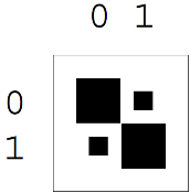
Example we take the joint distribution XY

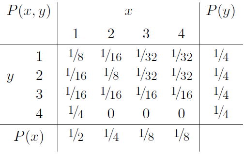
The marginal distributions P(x) and P(y) are shown in the margins. The joint entropy is H(X, Y) = 27/8 bits. The marginal entropies are H(X) = 7/4 bits and H(Y) = 2 bits.

Simple language models

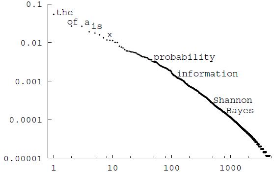
The Zipf-Mandelbrot distribution

The crudest model for a language is the monogram model, which asserts that each successive word is drawn independently from a distribution over words

Zipf's law (Zipf, 1949) asserts that the probability of the r^th most probable word in a language is approximately

Mandelbrot's (1982) modification of Zipf's law introduces a third parameter v, asserting that the probabilities are given by

Other documents give distributions that are not so well fitted by a Zipf–Mandelbrot distribution.

Soft K-means clustering

These criticisms of K-means motivate the ‘soft K-means algorithm’, algorithm. The algorithm has one parameter, β, which we could term the stiffness.

Algorithm. Soft K-means algorithm

Update step. The model parameters, the means, are adjusted to match the sample means of the data points that they are responsible for.

where R^(k) is the total responsibility of mean k,

Solving the decoding problems on a trellis

We can view the trellis of a linear code as giving a causal description of the probabilistic process that gives rise to a codeword, with time owing from left to right. Each time a divergence is encountered, a random source (the source of information bits for communication) determines which way we go.

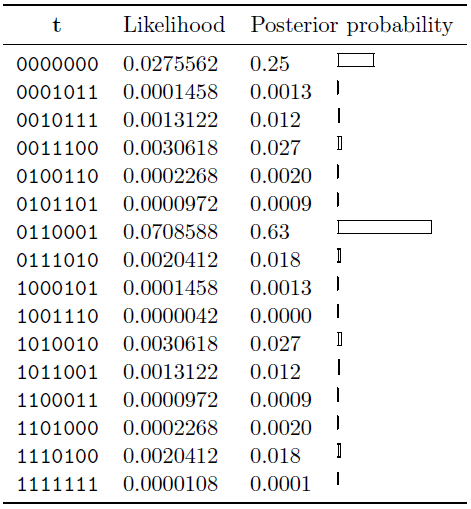
Example. Consider the case of a single transmission from the Hamming (7; 4) trellis shown in figure c.

Let the normalized likelihoods be: (0.1, 0.4, 0.9, 0.1, 0.1, 0.1, 0.3). That is, the ratios of the likelihoods are

We can find the posterior probability over codewords by explicit enumeration of all sixteen codewords. This posterior distribution is shown in table.

Source Models of discrete messages.

Message classification

Time

• continuous – stochastic time function;

• discrete – chain of stochastic events.

Set

• continuous – function may possess the range of values in an interval;

• discrete – may possess a finite set of discrete values.

Message classifications:

а) continuous in set and time

б) continuous in set, discrete in time

в) discrete in set, continuous in time

г) discrete in set and time

Symbol codes.

A symbol code is called a prefix code if no codeword is a prefix of any other codeword.

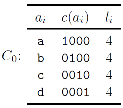
A (binary) symbol code C for an ensemble X is a mapping from the range of x, χ^N ={a₁,…,a_I}, to {0; 1}⁺. c(x) will denote the codeword corresponding to x, and l(x) will denote its length, with l_i = l(a_i).

The extended code C⁺ is a mapping from χ⁺ to {0, 1}⁺ obtained by concatenation

Example A symbol code for the ensemble X defined by

χ^N = {a, b, c, d}

P_X = {1/2, 1/4, 1/8, 1/8}

is C₀

The binary entropy function

the entropy of a random variable X is

Since this depends on p, this is also written sometimes as H(p).

Suppose X is a binary random variable,

Then the entropy of X is

Plot.

Observe:

concave function of p. (What does this mean?)

H(0) = 0, H(1) = 0

The burglar alarm

Bayesian probability theory is sometimes called “common sense, amplified”.

When thinking about the following questions, please ask your common sense what it thinks the answers are; we will then see how Bayesian methods confirm your everyday intuition.

P(b, e, a, p, r) = P(b)P(e)P(a | b, e)P(p | a)P(r | e)

and plausible values for the probabilities are:

1. Burglar probability:

P(b=1) = β, P(b=0) = 1 – β

e.g., β = 0.001 gives a mean burglary rate of once every three years.

2. Earthquake probability:

P(e=1) = ε, P(e=0) = 1 - ε

with, e.g., ε = 0.001, our assertion that the earthquakes are independent of burglars, i.e., the prior probability of b and e is P(b, e) = P(b)P(e), seems reasonable unless we take into account opportunistic burglars who strike immediately after earthquakes.

The capacity of a continuous channel of information transfer.

channel capacity is the tightest upper bound on the rate of information that can be reliably transmitted over a communications channel. By the noisy-channel coding theorem, the channel capacity of a given channel is the limiting information rate (in units of information per unit time) that can be achieved with arbitrarily small error probability

Let and be the random variables representing the input and output of the channel, respectively. Let be the conditional distribution function of given , which is an inherent fixed property of the communications channel. Then the choice of the marginal distribution completely determines the joint distribution due to the identity

which, in turn, induces a mutual information . The channel capacity is defined as

where the supremum is taken over all possible choices of .

The decoder

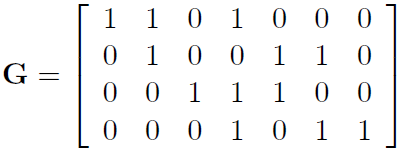
Decoding a sparse-graph code is especially easy in the case of an erasure channel.

The decoder's task is to recover s from t = Gs, where G is the matrix associated with the graph. The simple way to attempt to solve this problem is by message-passing.

This simplicity of the messages allows a simple description of the decoding process. We'll call the encoded packets {t_n} check nodes.

PRACTICE

1. Find a check node t_n that is connected to only one source packet s_k. (If there is no such check node, this decoding algorithm halts at this point, and fails to recover all the source packets.)

(a) Set s_k = t_n.

(b) Add s_k to all checks t_n' that are connected to s_k:

t_n' := t_n' + s_k for all n' such that G_n'k = 1.

(c) Remove all the edges connected to the source packet s_k.

.

The differential entropy and its properties.

Differential entropy (also referred to as continuous entropy) is a concept in information theory that extends the idea of (Shannon) entropy, a measure of average surprisal of a random variable, to continuous probability distributions.

Properties of differential entropy

• For two densities f and g, the Kullback-Leibler divergence D(f||g) is nonnegative with equality if f = g almost everywhere. Similarly, for two random variables X and Y, I(X;Y) ≥ 0 and h(X|Y) ≤ h(X) with equality if and only if X and Y are independent.

• The chain rule for differential entropy holds as in the discrete case

However, differential entropy does not have other desirable properties:

• It is not invariant under change of variables.

• It can be negative.

The entropy of a discrete source. Full and partial entropy.

In information theory, entropy is a measure of the uncertainty in a random variable.^[1] In this context, the term usually refers to the Shannon entropy, which quantifies the expected value of the information contained in a message.^[2] Entropy is typically measured in bits, nats, or bans.^[3] Shannon entropy is the average unpredictability in a random variable, which is equivalent to its information content

Named after Boltzmann's H-theorem, Shannon denoted the entropy H of a discrete random variable X with possible values {x₁, ..., x_n} and probability mass function P(X) as,

Here E is the expected value operator, and I is the information content of X.^[8][9] I(X) is itself a random variable.

When taken from a finite sample, the entropy can explicitly be written as

where b is the base of the logarithm used. Common values of b are 2, Euler's number e, and 10, and the unit of entropy is bit for b = 2, nat for b = e, and dit (or digit) for b = 10.^[10]

In the case of p(x_i) = 0 for some i, the value of the corresponding summand 0 log_b(0) is taken to be 0, which is consistent with the well-known limit:

.

The Gaussian channel

The most popular model of a real-input, real-output channel is the Gaussian channel.

The Gaussian channel has a real input x and a real output y. The conditional distribution of y given x is aGaussian distribution:

This channel has a continuous input and output but is discrete in time. We will show below that certain continuous-time channels are equivalent to the discrete-time Gaussian channel.

This channel is sometimes called the additive white Gaussian noise (AWGN) channel.

The general problem

Assume that a function P^* of a set of N variables is defined as a product of M factors as follows:

Each of the factors f_m(x_m) is a function of a subset x_m of the variables that make up x. If P* is a positive function then we may be interested in a second normalized function,

where the normalizing constant Z is defined by

As an example of the notation we've just introduced, here's a function of three binary variables x₁, x₂, x₃ defined by the five factors:

The information-retrieval problem

A simple example of an information-retrieval problem is the task of implementing a phone directory service, which, in response to a person's name, returns (a) a confirmation that that person is listed in the directory; and (b) the person's phone number and other details. We could formalize this problem as follows, with S being the number of names that must be stored in the directory.

The junction tree algorithm

What should one do when the factor graph one is interested in is not a tree?

There are several options, and they divide into exact methods and approximate methods. The most widely used exact method for handling marginalization on graphs with cycles is called the junction tree algorithm. This algorithm works by agglomerating variables together until the agglomerated graph has no cycles. You can probably figure out the details for yourself; the complexity of the marginalization grows exponentially with the number of agglomerated variables.

There are many approximate methods, however, the most amusing way of handling factor graphs to which the sum–product algorithm may not be applied is, as we already mentioned, to apply the sum–product algorithm! We simply compute the messages for each node in the graph, as if the graph were a tree and iterate.

The main types of signals used in the transmission of information.

Signals, or software interrupts, are external, asynchronous events used to alter the course of a program. These may occur at any time during the execution of a program. Because of this, they differ from other methods of inter-process communication, where two processes must be explicitly directed to wait for external messages; for example, by calling read on a pipe (see chapter 5).

The amount of information transmitted via a signal is minimal, just the type of signal, and although they were not originally intended for communication between processes, they do make it possible to transmit atomic information about the state of an external entity (e.g. the state of the system or another process).

The min–sum algorithm

The sum–product algorithm solves the problem of finding the marginal function of a given product P^*(x). This is analogous to solving the bitwise decoding problem. And just as there were other decoding problems (for example, the codeword decoding problem), we can define other tasks involving P^*(x) that can be solved by modifications of the sum–product algorithm.

The noisy-channel coding theorem (preparation)

It seems plausible that the “capacity” we have defined may be a measure of information conveyed by a channel; what is not obvious is that the capacity indeed measures the rate at which blocks of data can be communicated over the channel with arbitrarily small probability of error.

We make the following definitions.

An (N,K) block code for a channel Q is a list of S = 2^K codewords

each of length N. Using this code we can encode a signal as x^(s). [The number of codewords S is an integer, but the number of bits specified by choosing a codeword, K ≡ log₂S, is not necessarily an integer.]

The rate of the code is R = K/N bits per channel use. [We will use this definition of the rate for any channel, not only channels with binary inputs; note however that it is sometimes conventional to define the rate of a code for a channel with q input symbols to be K/(N log q).]

A decoder for an (N,K) block code is a mapping from the set of length-N strings of channel outputs, , to a codeword label

The extra symbol ŝ=0 can be used to indicate a ”failure”.

The probability of block error of a code and decoder, for a given channel, and for a given probability distribution over the encoded signal P(s_in), is:

The maximal probability of block error is

The optimal decoder for a channel code is the one that minimizes the probability of block error. It decodes an output y as the input s that has maximum posterior probability P(s | y).

A uniform prior distribution on s is usually assumed, in which case the optimal decoder is also the maximum likelihood decoder, i.e., the decoder that maps an output y to the input s that has maximum likelihood P(y | s).

The probability of bit error p_b is defined assuming that the codeword number s is represented by a binary vector s of length K bits; it is the average probability that a bit of s_out is not equal to the corresponding bit of s_in (averaging over all K bits).

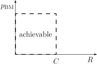
Shannon's noisy-channel coding theorem (part one). Associated with each discrete memoryless channel, there is a non-negative number C (called the channel capacity) with the following property. For any ε > 0 and R < C, for large enough N, there exists a block code of length N and rate ≥ R and a decoding algorithm, such that the maximal probability of block error is < ε.

The set, which objects of an information transmission system?

An information transmission network in which a plurality of information processing stations are connected in parallel to a bus line is disclosed. Each station has a communication control means and an information processor. Each control means is capable of establishing command over the bus line to the exclusion of all other stations. While command is established, the commanding station can communicate with all other stations. After one sequence of communication, command is transferred. If the station presently in command fails, the failure to transfer command in a predetermined time will be noted and another station with highest priority will assume command. If the station to which command is transferred is not operating properly, the station presently in command will detect a failure of the former station to respond to transfer of command and will thereupon transfer command to another station.

The sum–product algorithm

Notation

We identify the set of variables that the mth factor depends on, x_m, by the set of their indices N(m). For our example, the sets are N(1) = {1} (since f₁ is a function of x₁ alone), N(2) = {2}, N(3) = {3}, N(4) = {1, 2}, and N(5) = {2, 3}. Similarly we define the set of factors in which variable n participates, by M(n). We denote a set N(m) with variable n excluded by N(m)\n. We introduce the shorthand x_m\n or x_m\n to denote the set of variables in x_m with x_n excluded, i.e.,

The sum–product algorithm will involve messages of two types passing along the edges in the factor graph: messages q_n→m from variable nodes to factor nodes, and messages r_m→n from factor nodes to variable nodes. A message (of either type, q or r) that is sent along an edge connecting factor f_m to variable x_n is always a function of the variable x_n.

Here are the two rules for the updating of the two sets of messages.

From variable to factor:

From factor to variable:

Turbo codes

An (N,K) turbo code is defined by a number of constituent convolutional encoders (often, two) and an equal number of interleavers which are K × K permutation matrices. Without loss of generality, we take the first interleaver to be the identity matrix. A string of K source bits is encoded by feeding them into each constituent encoder in the order defined by the associated interleaver, and transmitting the bits that come out of each constituent encoder. Often the first constituent encoder is chosen to be a systematic encoder, just like the recursive filter, and the second is a non-systematic one of rate 1 that emits parity bits only. The transmitted codeword then consists of K source bits followed by M₁ parity bits generated by the first convolutional code and M₂ parity bits from the second. The resulting turbo code has rate 1/3.

Each box C₁, C₂, contains a convolutional code.

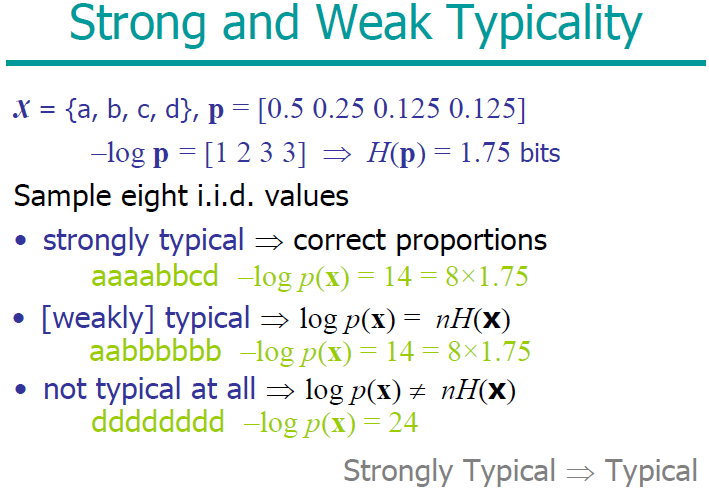
Typicality

Let us define typicality for an arbitrary ensemble X with alphabet χ. Our definition of a typical string will involve the string's probability. A long string of N symbols will usually contain about p₁N occurrences of the first symbol, p₂N occurrences of the second, etc. Hence the probability of this string is roughly

so that the information content of a typical string is

So the random variable log₂1/P(x), which is the information content of x, is very likely to be close in value to NH. We build our definition of typicality on this observation.

Units of information content

The information content of an outcome, x, whose probability is P(x), is defined to be

The entropy of an ensemble is an average information content,

When we compare hypotheses with each other in the light of data, it is often convenient to compare the log of the probability of the data under the alternative hypotheses,

`log evidence for H_i' = log P(D | H_i)

or, in the case where just two hypotheses are being compared, we evaluate the `log odds',

which has also been called the `weight of evidence in favour of H₁'. The log evidence for a hypothesis, log P(D|H_i) is the negative of the information content of the data D: if the data have large information content, given a hypothesis, then they are surprising to that hypothesis; if some other hypothesis is not so surprised by the data, then that hypothesis becomes more probable.

What are the capabilities of practical error-correcting codes?

Nearly all codes are good, but nearly all codes require exponential look-up tables for practical implementation of the encoder and decoder – exponential in the blocklength N. And the coding theorem required N to be large.

By a practical error-correcting code, we mean one that can be encoded and decoded in a reasonable amount of time, for example, a time that scales as a polynomial function of the blocklength N – preferably linearly.

What are the main problems of the theory of information

The central paradigm of classical information theory is the engineering problem of the transmission of information over a noisy channel. The most fundamental results of this theory are Shannon's source coding theorem, which establishes that, on average, the number of bits needed to represent the result of an uncertain event is given by its entropy; and Shannon's noisy-channel coding theorem, which states that reliable communication is possible over noisy channels provided that the rate of communication is below a certain threshold, called the channel capacity. The channel capacity can be approached in practice by using appropriate encoding and decoding systems.

What are the main stages of treatment information?(ZDES” NIGDE NETU SLOVA TREATMENT vo vseh 15 slaidah I v NETE!! Pohodu on pereputal s Transmission???)

. On the stage of information transmission and storage – information is being transmitted form source to destination (in space and time). Mechanisms and problems of information transmission and storage are very coherent to each other. For that purposes different physical environment could be used (electric, electro-magnetic, optic, etc.).

What Information system is?

Information Systems (IS) is a professional and academic discipline concerned with the strategic, managerial and operational activities involved in the gathering, processing, storing, distributing and use of information, and its associated technologies, in society and organizations. This systems could be tightly coupled, sonar, navigation, TV, calculation, measurement, automation control systems etc

What is meant by the message and the signal?

Message is a set of characters or other initial signals that contains an amount of information.Transmitter - transform message into signals code message;modulate; Signal is a material message transmitter.

What is said to be centered random process?

X⁰(t)=X(t)-m_X(t) центрированный случайный процесс.(bol’we nikokoi informacii netu pro eto proveril 4 sourca)

What is the difference between a line and a channel of communication?

In telecommunications and computer networking, a communication channel, or channel, refers either to a physical transmission medium such as a wire, or to a logical connection over a multiplexed medium such as a radio channel. A channel is used to convey an information signal, for example a digital bit stream, from one or several senders (or transmitters) to one or several receivers. A channel has a certain capacity for transmitting information, often measured by its bandwidth in Hz or its data rate in bits per second.

LINE Communications is a privately held, European-based blended learning and communications solution company. LINE is recognised by the British Computer Society as the UK market leader in bespoke e-learning content development

What is the difficulty of exact mathematical description of a random process?

Intuitively, we might want any measure of the `amount of information gained' to have the property of additivity – that is, for independent random variables x and y, the information gained when we learn x and y should equal the sum of the information gained if x alone were learned and the information gained if y alone were learned.

The Shannon information content of the outcome x; y is

so it does indeed satisfy if x and y are independent.

(VATA POLNAYA)

What is the essence of fundamental differences in the interpretation of the concept of information?

The concept of information as we use it in everyday English in the sense knowledge communicated plays a central role in today's society. The concept became particularly predominant since end of World War II with the widespread use of computer networks. The rise of information science in the middle fifties is a testimony of this. For a science like information science (IS) it is of course important how its fundamental terms are defined, and in IS as in other fields the problem of how to define information is often raised. This review is an attempt to overview the present status of the information concept in IS with a view also to interdisciplinary trends.

What limit is imposed by unique decode ability?

We now ask, given a list of positive integers {l_i}, does there exist a uniquely decodable code with those integers as its codeword lengths? At this stage, we ignore the probabilities of the different symbols; once we understand unique decodeability better, we'll reintroduce the probabilities and discuss how to make an optimal uniquely decodable symbol code.(4week)

What's the most compression that we can hope for?

We wish to minimize the expected length of a code,

As you might have guessed, the entropy appears as the lower bound on the expected length of a code.Lower bound on expected length. The expected length L(C,X) of a uniquely decodable code is bounded below by H(X).

The equality L(C,X) =H(X) is achieved only if the Kraft equality z =1 is satisfied, and if the codelengths satisfy l_i=log₂(1/p_i).

This is an important result so let's say it again:Optimal source codelengths. The expected length is minimized and is equal to H(X) only if the codelengths are equal to the Shannon information contents l_i=log₂(1/p_i)Implicit probabilities defined by codelengths. Conversely, any choice of codelengths {l_i} implicitly defines a probability distribution {q_i},

for which those codelengths would be the optimal codelengths. If the code is complete then z = 1 and the implicit probabilities are given by