A digital fountain's encoder

The encoding algorithm produces an droplet, v, from a number of source

segments. The number of source segments used to produce a droplet is

called the degree, and this is chosen at random from a previously determined

degree distribution.

This encoding operation defines a graph connecting encoded packets to source packets. If the mean degree is significantly smaller than K then the graph is sparse. We can think of the resulting code as an irregular low-density generator-matrix code.

For example, if the sender and receiver have synchronized clocks, they could use identical pseudo-random number generators, seeded by the clock, to choose each random degree and each set of connections. Alternatively, the sender could pick a random key, k_n, given which the degree and the connections are determined by a pseudorandom process, and send that key in the header of the packet. As long as the packet size l is much bigger than the key size (which need only be 32 bits or so), this key introduces only a small overhead cost.

A fatal flaw of maximum likelihood

Example:when we fit K = 4 means to our first toy data set, we sometimes find that very small clusters form, covering just one or two data points. This is a pathological property of soft K-means clustering, versions 2 and 3.

A popular replacement for maximizing the likelihood is maximizing the Bayesian posterior probability density of the parameters instead. However, multiplying the likelihood by a prior and maximizing the posterior does not make the above problems go away; the posterior density often also has infinitely-large spikes, and the maximum of the posterior probability density is often unrepresentative of the whole posterior distribution. Think back to the concept of typicality: in high dimensions, most of the probability mass is in a typical set whose properties are quite different from the points that have the maximum probability density. Maxima are atypical.

A further reason for disliking the maximum a posteriori is that it is basis-dependent. If we make a nonlinear change of basis from the parameter θ to the parameter u = f(θ) then the probability density of θ is transformed to

The maximum of the density P(u) will usually not coincide with the maximum of the density P(θ).

It seems undesirable to use a method whose answers change when we change representation.

A taste of Banburismus

The details of the code-breaking methods of Bletchley Park were kept secret for a long time, but some aspects of Banburismus can be pieced together.

How much information was needed? The number of possible settings of the Enigma machine was about 8×10¹². To deduce the state of the machine, `it was therefore necessary to find about 129 decibans from somewhere', as Good puts it. Banburismus was aimed not at deducing the entire state of the machine, but only at figuring out which wheels were in use; the logic-based bombes, fed with guesses of the plaintext (cribs), were then used to crack what the settings of the wheels were.

The Enigma machine, once its wheels and plugs were put in place, implemented a continually-changing permutation cypher that wandered deterministically through a state space of 26³ permutations. Because an enormous number of messages were sent each day, there was a good chance that whatever state one machine was in when sending one character of a message, there would be another machine in the same state while sending a particular character in another message.

Amount of information. Basic properties of information.

Message is a set of characters or other initial signals that contains an amount of information.

New knowledge about environment;

It could be collected in collaboration with that environment; in adaptation to that environment;

Arithmetic codes

When we discussed variable-length symbol codes, and the optimal Huffman algorithm for constructing them, we concluded by pointing out two practical and theoretical problems with Huffman codes.

Example: compressing the tosses of a bent coin

Capacity of Gaussian channel

Until now we have measured the joint, marginal, and conditional entropy of discrete variables only. In order to define the information conveyed by continuous variables, there are two issues we must address – the infinite length of the real line, and the infinite precision of real numbers.

Additive white Gaussian noise (AWGN) is a channel model in which the only impairment to communication is a linear addition of wideband or white noise with a constant spectral density (expressed as watts per hertz of bandwidth) and a Gaussian distribution of amplitude.

The AWGN channel is represented by a series of outputs at discrete time event index . is the sum of the input and noise, , where is independent and identically distributed and drawn from a zero-mean normal distribution with variance (the noise). The are further assumed to not be correlated with the .

The capacity of the channel is infinite unless the noise n is nonzero, and the are sufficiently constrained. The most common constraint on the input is the so-called "power" constraint, requiring that for a codeword transmitted through the channel, we have:

where represents the maximum channel power. Therefore, the channel capacity for the power-constrained channel is given by:

W here is the distribution of . Expand , writing it in terms of the differential entropy:

But and are independent, therefore:

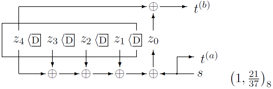
Codes and trellises

Linear (N,K) codes could be represented in terms of their generator matrices and their parity-check matrices. In the case of a systematic block code, the first K transmitted bits in each block of size N are the source bits, and the remaining M = N – K bits are the parity-check bits. This means that the generator matrix of the code can be written

and the parity-check matrix can be written

where P is an M × K matrix.

Here we will study another representation of a linear code called a trellis. The codes that these trellises represent will not in general be systematic codes, but they can be mapped onto systematic codes if desired by a reordering of the bits in a block.

A trellis is a graph consisting of nodes (also known as states or vertices) and edges. The nodes are grouped into vertical slices called times, and the times are ordered such that each edge connects a node in one time to a node in a neighbouring time.

Example:

(a) Repetition code R3

(b) Simple parity code P3

Coding and Modulation in data transmission systems.

Coding and modulation provide the means of mapping information into waveforms such that the receiver (with an appropriate demodulator and decoder) can recover the information in a reliable manner. The simplest model for a communication system is that of an additive white Gaussian noise (AWGN) system. In this model a user transmits information by sending one of M possible waveforms in a given time, period T, with a given amount of energy. The rate of communication, R, in bits per second is log₂(M)/T. The signal occupies a given bandwidth W Hz. The normalized rate of communications is R/W measured in bits/second/Hz.

Data transmission, digital transmission, or digital communications is the physical transfer of data (a digital bit stream) over a point-to-point or point-to-multipoint communication channel. Examples of such channels are copper wires, optical fibres, wireless communication channels, and storage media. The data are represented as an electromagnetic signal, such as an electrical voltage, radiowave, microwave, or infrared signal.

Collision resolution

We will study two ways of resolving collisions: appending in the table, and storing elsewhere.

Appending in table

When encoding, if a collision occurs, we continue down the hash table and write the value of s into the next available location in memory that currently contains a zero. If we reach the bottom of the table before encountering a zero, we continue from the top.

For this method, it is essential that the table be substantially bigger in size than S. If 2^M < S then the encoding rule will become stuck with nowhere to put the last strings.

Storing elsewhere

As an example, we could store in location h in the hash table a pointer (which must be distinguishable from a valid record number s) to a “bucket” where all the strings that have hash code h are stored in a sorted list. The encoder sorts the strings in each bucket alphabetically as the hash table and buckets are created.

This method of storing the strings in buckets allows the option of making the hash table quite small, which may have practical benefit

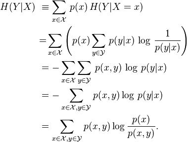
Conditional entropy and its properties.

In information theory, the conditional entropy (or equivocation) quantifies the amount of information needed to describe the outcome of a random variable given that the value of another random variable is known. Here, information is measured in bits, nats, or bans. The entropy of conditioned on is written as .

Given discrete random variable with support and with support , the conditional entropy of given is defined as:

Convexity and Jensen's inequality

A large part of information theory consists in finding bounds on certain performance measures. The analytical idea behind a bound is to substitute a complicated expression for something simpler but not exactly equal, known to be either greater or smaller than the thing it replaces. This gives rise to simpler statements (and hence gain some insight), but usually at the expense of precision.

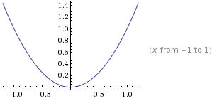
A function f(x) is said to be convex over an interval (a,b) if for every and ,

A function is strictly convex if equality holds only if or .

Convex

Concave:

Theorem 8 , with equality if and only if p(x) = q(x) for all x.

Proof

Data compression

The preceding examples justify the idea that the Shannon information content of an outcome is a natural measure of its information content. Improbable outcomes do convey more information than probable outcomes. We now discuss the information content of a source by considering how many bits are needed to describe the outcome of an experiment. If we can show that we can compress data from a particular source into a file of L bits per source symbol and recover the data reliably, then we will say that the average information content of that source is at most L bits per symbol.

Some simple data compression methods that define measures of information content

Example

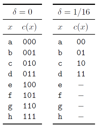
The raw bit content of this ensemble is 3 bits, corresponding to 8 binary names. But notice that . So if we are willing to run a risk of of not having a name for x, then we can get by with four names – half as many names as are needed if every x has a name.

Decoding convolutional codes

The receiver receives a bit stream, and wishes to infer the state sequence and thence the source stream. The posterior probability of each bit can be found by the sum–product algorithm (also known as the forward–backward or BCJR algorithm). The most probable state sequence can be found using the min–sum algorithm (also known as the Viterbi algorithm).

Decoding problems

A codeword t is selected from a linear (N,K) code C, and it is transmitted over a noisy channel; the received signal is y. Here we will assume that the channel is a memoryless channel such as a Gaussian channel. Given an assumed channel model P(y | t), there are two decoding problems.

The codeword decoding problem is the task of inferring which codeword t was transmitted given the received signal.

The bitwise decoding problem is the task of inferring for each transmitted bit t_n how likely it is that that bit was a one rather than a zero.

As a concrete example, take the (7; 4) Hamming code. We discussed the codeword decoding problem for that code, assuming a binary symmetric channel. We didn't discuss the bitwise decoding problem and we didn't discuss how to handle more general channel models such as a Gaussian channel.

Solving the codeword decoding problem

By Bayes' theorem, the posterior probability of the codeword t is

Decoding with the sum–product algorithm

We aim, given the observed checks, to compute the marginal posterior probabilities P(x_n =1 | z,H) for each n. It is hard to compute these exactly because the graph contains many cycles. However, it is interesting to implement the decoding algorithm that would be appropriate if there were no cycles, on the assumption that the errors introduced might be relatively small. Cost. In a brute-force approach, the time to create the generator matrix scales as N³, where N is the block size. The encoding time scales as N², but encoding involves only binary arithmetic, so for the block lengths studied here it takes considerably less time than the simulation of the Gaussian channel.

Decoding involves approximately 6Nj floating-point multiplies per iteration, so the total number of operations per decoded bit (assuming 20 iterations) is about 120t/R, independent of blocklength.

The encoding complexity can be reduced by clever encoding tricks.

The decoding complexity can be reduced, with only a small loss in performance, by passing low-precision messages in place of real numbers.

Definition of the typical set

Let us define typicality for an arbitrary ensemble X with alphabet χ. Our definition of a typical string will involve the string's probability. A long string of N symbols will usually contain about p₁N occurrences of the first symbol, p₂N occurrences of the second, etc. Hence the probability of this string is roughly

so that the information content of a typical string is

Why did we introduce the typical set?

The best choice of subset for block compression is (by definition) S_δ, not a typical set. So why did we bother introducing the typical set? The answer is, we can count the typical set. We know that all its elements have “almost identical” probability (2^-NH), and we know the whole set has probability almost 1, so the typical set must have roughly 2^NH elements. Without the help of the typical set (which is very similar to S_δ) it would have been hard to count how many elements there are in S_δ.

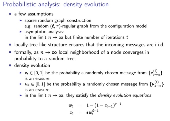
Density evolution

density evolution

is used in

I

analyzing channel codes

I

analyzing solution space of XORSAT

I

analyzing a message-passing algorithm for crowdsourcing

I

etc

Describe the disadvantages of the Huffman code.

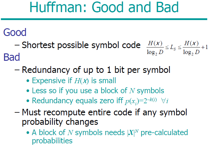
The Huffman algorithm produces an optimal symbol code for an ensemble, but this is not the end of the story. Both the word “ensemble” and the phrase “symbol code” need careful attention.

Changing ensemble

If we wish to communicate a sequence of outcomes from one unchanging ensemble, then a Huffman code may be convenient. But often the appropriate ensemble changes. If for example we are compressing text, then the symbol frequencies will vary with context: in English the letter u is much more probable after a q than after an e. And furthermore, our knowledge of these context-dependent symbol frequencies will also change as we learn the statistical properties of the text source.

The extra bit

An equally serious problem with Huffman codes is the innocuous-looking extra bit relative to the ideal average length of H(X) – a Huffman code achieves a length that satisfies H(X) ≤ L(C,X) < H(X) + 1

A Huffman code thus incurs an overhead of between 0 and 1 bits per symbol.

Beyond symbol codes

Huffman codes, therefore, although widely trumpeted as “optimal”, have many defects for practical purposes. They are optimal symbol codes, but for practical purposes we don't want a symbol code. The defects of Huffman codes are rectified by arithmetic coding, which dispenses with the restriction that each symbol must translate into an integer number of bits.

Describe the Lempel–Ziv coding.

The Lempel-Ziv algorithms, which are widely used for data compression (e.g., the compress and gzip commands), are different in philosophy to arithmetic coding. There is no separation between modelling and coding, and no opportunity for explicit modelling.

Example Encode the string 000000000000100000000000 using the basic Lempel-Ziv algorithm described above.

The encoding is 010100110010110001100, which comes from the parsing

0, 00, 000, 0000, 001, 00000, 000000

which is encoded thus:

(, 0), (1, 0), (10, 0), (11, 0), (010, 1), (100, 0), (110, 0)

Decode the string 00101011101100100100011010101000011 that was encoded using the basic Lempel-Ziv algorithm.

The decoding is 0100001000100010101000001

Describe the main research method signals.

Research in common parlance refers to a search for knowledge. Once can also define research as

a scientific and systematic search for pertinent information on a specific topic. In fact, research is an

art of scientific investigation.

Describe the Noisy-Channel coding theorem (extended).

The Noisy-Channel Coding Theorem (extended)

The theorem has three parts, two positive and one negative.

1. For every discrete memoryless channel, the channel capacity

has the following property. For any ε > 0 and R < C, for large enough N, there exists a code of length N and rate ≥ R and a decoding algorithm, such that the maximal probability of block error is < ε.

2. If a probability of bit error p_b is acceptable, rates up to R(p_b) are achievable, where

3. For any p_b, rates greater than R(p_b) are not achievable.

Describe the types of information systems and their development.

1. knowledge area (biologic, industry, financial, etc)

2. physical nature (acoustic, visual, gustatory)

3. Structural-measurement properties.

Parametric information – contains numerical evaluation of different properties.

Information types	Key	Information representation form
		Topologic	Abstract	Linguistic
event value function complex ................ field	Ф0 Ф1 Ф2 Ф3 ......... Фn	point line surface volume .............. dimension	opinion idea image system ............. universe	sign character word sentence ............... fund

Designing the degree distribution

The probability distribution ρ(d) of the degree is a critical part of the design: occasional encoded packets must have high degree (i.e., d similar to K) in order to ensure that there are not some source packets that are connected to no-one. , to avoid redundancy, we'd like the received graph to have the property that just one check node has degree one at each iteration. At each iteration, when this check node is processed, the degrees in the graph are reduced in such a way that one new degree-one check node appears. In expectation, this ideal behaviour is achieved by the ideal soliton distribution,

The expected degree under this distribution is roughly lnK.

Digital Fountain Codes

Common methods for communicating over such channels employ a feedback channel from receiver to sender that is used to control the retransmission of erased packets. For example, the receiver might send back messages that identify the missing packets, which are then retransmitted. Alternatively, the receiver might send back messages that acknowledge each received packet; the sender keeps track of which packets have been acknowledged and retransmits the others until all packets have been acknowledged.

These simple retransmission protocols have the advantage that they will work regardless of the erasure probability f, but purists who have learned their Shannon theory will feel that these retransmission protocols are wasteful. If the erasure probability f is large, the number of feedback messages sent by the first protocol will be large. Under the second protocol, it's likely that the receiver will end up receiving multiple redundant copies of some packets, and heavy use is made of the feedback channel. According to Shannon, there is no need for the feedback channel: the capacity of the forward channel is (1 – f)l bits, whether or not we have feedback.

Efficient coding. Shannon coding in the channel without interference. –

In the field of data compression, Shannon–Fano coding, named after Claude Shannon and Robert Fano, is a technique for constructing a prefix code based on a set of symbols and their probabilities (estimated or measured). It is suboptimal in the sense that it does not achieve the lowest possible expected code word length like Huffman coding; however unlike Huffman coding, it does guarantee that all code word lengths are within one bit of their theoretical ideal . The technique was proposed in Shannon's "A Mathematical Theory of Communication", his 1948 article introducing the field of information theory. The method was attributed to Fano, who later published it as a technical report.^[1] Shannon–Fano coding should not be confused with Shannon coding, the coding method used to prove Shannon's noiseless coding theorem, or with Shannon–Fano–Elias coding (also known as Elias coding), the precursor to arithmetic coding.

In Shannon–Fano coding, the symbols are arranged in order from most probable to least probable, and then divided into two sets whose total probabilities are as close as possible to being equal. All symbols then have the first digits of their codes assigned;

Enhancements to soft K-means

Algorithm is a version 2 of the soft-K-means algorithm corresponding to a modelling assumption that each cluster is a spherical Gaussian having its own width (each cluster has its own β^(k) = 1/σ_k²). The algorithm updates the lengthscales σ_k for itself. The algorithm also includes cluster weight parameters π₁, π₂,…, π_K which also update themselves, allowing accurate modelling of data from clusters of unequal weights.

Entropy. Basic properties of entropy.

In information theory, entropy is a measure of the uncertainty in a random variable.^[1] In this context, the term usually refers to the Shannon entropy, which quantifies the expected value of the information contained in a message.^[2] Entropy is typically measured in bits, nats, or bans.^[3] Shannon entropy is the average unpredictability in a random variable, which is equivalent to its information content. The concept was introduced by Claude E. Shannon in his 1948 paper "A Mathematical Theory of Communication".^[4] Shannon entropy provides an absolute limit on the best possible lossless encoding or compression of any communication, assuming that^[5] the communication may be represented as a sequence of independent and identically distributed random variables. Shannon's source coding theorem shows that, in the limit, the average length of the shortest possible representation to encode the messages in a given alphabet is their entropy divided by the logarithm of the number of symbols in the target alphabet

Exact inference for continuous hypothesis spaces

Many of the hypothesis spaces we will consider are naturally thought of as continuous. For example, the unknown decay length of section 3.1 (p. 48) lives in a continuous one-dimensional space; and the unknown mean and standard deviation of a Gaussian ; live in a continuous two-dimensional space. In any practical computer implementation, such continuous spaces will necessarily be discretized however, and so can, in principle, be enumerated {at a grid of parameter values, for example.

Explain the difference in the levels of communication problems. Kto-to sxal9vil etot vopros

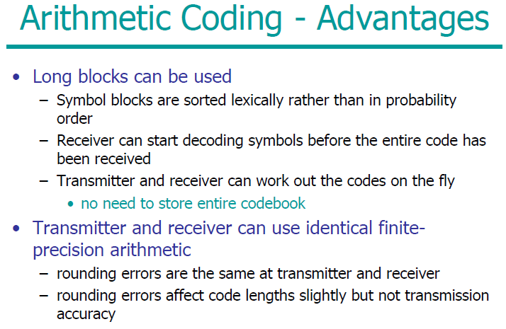
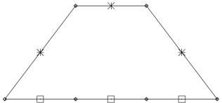
Finding the lowest-cost path

Imagine you wish to travel as quickly as possible from Almaty (A) to Bishkek (B). The various possible routes are shown in figure, along with the cost in hours of traversing each edge in the graph. For example, the route A-I-L-N-B has a cost of 8 hours.

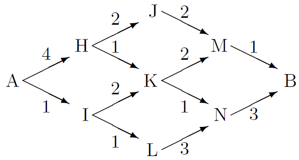
We would like to find the lowest-cost path without explicitly evaluating the cost of all paths. We can do this efficiently by finding for each node what the cost of the lowest-cost path to that node from A is. These quantities can be computed by message-passing, starting from node A. The message-passing algorithm is called the min-sum algorithm or Viterbi algorithm.

Functional diagram of the transmission of information, the purpose of its components.

Data transmission, digital transmission, or digital communications is the physical transfer of data (a digital bit stream) over a point-to-point or point-to-multipoint communication channel. Examples of such channels are copper wires, optical fibres, wireless communication channels, and storage media. The data are represented as an electromagnetic signal, such as an electrical voltage, radiowave, microwave, or infrared signal.

While analog transmission is the transfer of a continuously varying analog signal, digital communications is the transfer of discrete messages. The messages are either represented by a sequence of pulses by means of a line code (baseband transmission), or by a limited set of continuously varying wave forms (passband transmission), using a digital modulation method. The passband modulation and corresponding demodulation (also known as detection) is carried out by modem equipment. According to the most common definition of digital signal, both baseband and passband signals representing bit-streams are considered as digital transmission, while an alternative definition only considers the baseband signal as digital, and passband transmission of digital data as a form of digital-to-analog conversion.

Data transmitted may be digital messages originating from a data source, for example a computer or a keyboard. It may also be an analog signal such as a phone call or a video signal, digitized into a bit-stream for example using pulse-code modulation (PCM) or more advanced source coding (analog-to-digital conversion and data compression) schemes. This source coding and decoding is carried out by codec equipment.

Further applications of arithmetic coding

Arithmetic coding not only offers a way to compress strings believed to come from a given model; it also offers a way to generate random strings from a model. Imagine sticking a pin into the unit interval at random, that line having been divided into subintervals in proportion to probabilities p_i; the probability that your pin will lie in interval i is p_i.

So to generate a sample from a model, all we need to do is feed ordinary random bits into an arithmetic decoder for that model. An infinite random bit sequence corresponds to the selection of a point at random from the line [0, 1), so the decoder will then select a string at random from the assumed distribution. This arithmetic method is guaranteed to use very nearly the smallest number of random bits possible to make the selection – an important point in communities where random numbers are expensive! [This is not a joke. Large amounts of money are spent on generating random bits in software and hardware. Random numbers are valuable.]

A simple example of the use of this technique is in the generation of random bits with a nonuniform distribution {p₀,p₁}.

Example Compare the following two techniques for generating random symbols from a nonuniform distribution {p₀,p₁} = {0.99, 0.01}

Gaussian distribution

One-dimensional Gaussian distribution.

If a random variable y is Gaussian and has mean μ and variance σ², which we write:

y ~ Normal(μ, σ²); or P(y) = Normal(y, μ, σ²)

then the distribution of y is:

The inverse-variance τ ≡ 1/ σ² is sometimes called the precision of the Gaussian distribution.

Multi-dimensional Gaussian distribution.

If y = (y₁, y₂, . . . , y_N) has a multivariate Gaussian distribution, then

where x is the mean of the distribution, A is the inverse of the variance–covariance matrix, and the normalizing constant is Z(A) = (det(A/2π))^-1/2.

This distribution has the property that the variance Σ_ii of y_i, and the covariance Σ_ij of y_i and y_j are given by

where A^-1 is the inverse of the matrix A.

The marginal distribution P(y_i) of one component y_i is Gaussian; the joint marginal distribution of any subset of the components is multivariate-Gaussian; and the conditional density of any subset, given the values of another subset, for example, P(y_i | y_j), is also Gaussian.

Generalized parity-check matrices

can be used to define systematic linear block codes for Single Error Correction-Double Error Detection (SEC-DED). Their fixed code word parity enables the construction of low density parity-check matrices and fast hardware implementations. Fixed code word parity is enabled by an all-one row in extended Hamming parity-check matrices or by the constraint that the modulo-2 sum of all rows is equal to the all-zero vector in Hsiao parity-check matrices.

Give the definition of a stationary random process in the narrow and broad sense.

In mathematics, a stationary process (or strict(ly) stationary process or strong(ly) stationary process) is a stochastic process whose joint probability distribution does not change when shifted in time or space. Consequently, parameters such as the mean and variance, if they exist, also do not change over time or position.

Stationarity is used as a tool in time series analysis, where the raw data are often transformed to become stationary; for example, economic data are often seasonal and/or dependent on a non-stationary price level. An important type of non-stationary process that does not include a trend-like behavior is the cyclostationary process.

Note that a "stationary process" is not the same thing as a "process with a stationary distribution".^{[clarification needed]} Indeed there are further possibilities for confusion with the use of "stationary" in the context of stochastic processes; for example a "time-homogeneous" Markov chain is sometimes said to have "stationary transition probabilities". On the other hand, all stationary Markov random processes are time-homogeneous.

Hash codes

First we will describe how a hash code works, then we will study the properties of idealized hash codes. A hash code implements a solution to the information retrieval problem, that is, a mapping from x to s, with the help of a pseudorandom function called a hash function, which maps the N-bit string x to an M-bit string h(x), where M is smaller than N. M is typically chosen such that the “table size” T ≈ 2^M is a little bigger than S – say, ten times bigger. For example, if we were expecting S to be about a million, we might map x into a 30-bit hash h (regardless of the size N of each item x). The hash function is some fixed deterministic function which should ideally be indistinguishable from a fixed random code. For practical purposes, the hash function must be quick to compute.

How much can we compress?

So, we can't compress below the entropy. How close can we expect to get to the entropy?

Theorem Source coding theorem for symbol codes. For an ensemble X there exists a prefix code C with expected length satisfying H(X) ≤ L(C,X) < H(X) + 1

Proof. We set the codelengths to integers slightly larger than the optimum lengths:

where denotes the smallest integer greater than or equal to l^*. [We are not asserting that the optimal code necessarily uses these lengths, we are simply choosing these lengths because we can use them to prove the theorem.]

We check that there is a prefix code with these lengths by confirming that the Kraft inequality is satisfied.

Then we confirm

How to measure the information content of a random variable?

1.Shannon information content,

is a sensible measure of the information content of the outcome x = a_i

2. the entropy of the ensemble,

is a sensible measure of the ensemble's average information content.

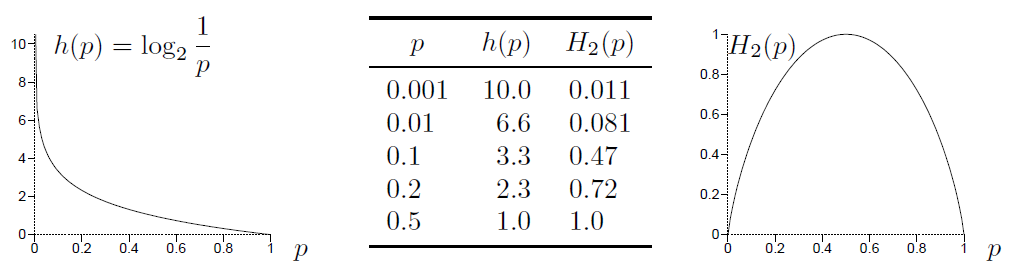
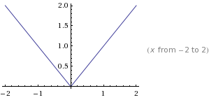
The Shannon information content h(p) = log₂(p) and the binary entropy function

as a function of p. The less probable an outcome is, the greater its Shannon information content.

Inferring the input to a real channel

In 1944 Shannon wrote a memorandum on the problem of best differentiating between two types of pulses of known shape, represented by vectors x₀ and x₁, given that one of them has been transmitted over a noisy channel. This is a pattern recognition problem. It is assumed that the noise is Gaussian with probability density

The probability of the received vector y given that the source signal was s (either zero or one) is then

The optimal detector is based on the posterior probability ratio:

If the detector is forced to make a decision (i.e., guess either s=1 or s=0) then the decision that minimizes the probability of error is to guess the most probable hypothesis. We can write the optimal decision in terms of a discriminant function:

with the decisions

a(y) > 0 → guess s=1

a(y) < 0 → guess s=0

a(y) = 0 → guess either.

Inferring the mean and variance of a Gaussian distribution

We discuss again the one-dimensional Gaussian distribution, parameterized by a mean μ and a standard deviation σ:

When inferring these parameters, we must specify their prior distribution. The prior gives us the opportunity to include specific knowledge that we have about μ and σ (from independent experiments, or on theoretical grounds, for example). If we have no such knowledge, then we can construct an appropriate prior that embodies our supposed ignorance. We assume a uniform prior over the range of parameters plotted. If we wish to be able to perform exact marginalizations, it may be useful to consider conjugate priors; these are priors whose functional form combines naturally with the likelihood such that the inferences have a convenient form.

Conjugate priors for μ and σ

The conjugate prior for a mean μ is a Gaussian: we introduce two `hyper-parameters', μ₀ and σ_μ, which parameterize the prior on μ, and write P(μ | μ₀; σ_μ) = Normal(μ; μ₀, σ_μ²). In the limit μ₀ =0, σ_μ→∞, we obtain the non-informative prior for a location parameter, the flat prior. This is non-informative because it is invariant under the natural re-parameterization μ' = μ+c. The prior P(μ) = const: is also an improper prior, that is, it is not normalizable.

The conjugate prior for a standard deviation σ is a gamma distribution, which has two parameters b_β and c_β. It is most convenient to define the prior density of the inverse variance (the precision parameter) β = 1/σ²:

This is a simple peaked distribution with mean b_βc_β and variance b_β²c_β. In the limit b_βc_β = 1; c_β → ∞, we obtain the non-informative prior for a scale parameter, the 1/ σ prior. This is `non-informative' because it is invariant under the re-parameterization σ' = cσ. The 1/ σ prior is less strange-looking if we examine the resulting density over ln σ, or ln β, which is flat. This is the prior that expresses ignorance about σ by saying ‘well, it could be 10, or it could be 1, or it could be 0.1, . . .’ Scale variables such as σ are usually best represented in terms of their logarithm. Again, this non-informative 1/σ prior is improper.

Reminder: when we change variables from σ to l(σ), a one-to-one function of σ, the probability density transforms from P_σ(σ) to

Here, the Jacobian is

In the following examples, we will use the improper non-informative priors for σ and μ. Using improper priors is viewed as distasteful in some circles, let us say it's for the sake of simplicity; if we include proper priors, the calculations could still be done but the key points would be obscured by the flood of extra parameters.