S

Fig. 12. Porosity fields displayed at different depth in the 2d Geometry plot

imulation: Run Settings and Problem initialization

Run Settings

For defining duration of simulation I open “Simulation – Run Settings” dialog, check the “Run for” flag and input 1000 days in the first tab.

Initialization

After clicking on “Initialize” button in the “Simulation” page initial state of formation is computed. Pressure and saturation properties are shown on the 3D plot and Cross-Section plot (Fig. 13,14,15).

F ig. 14. Initial saturations field displayed in the 3D Geometry plot

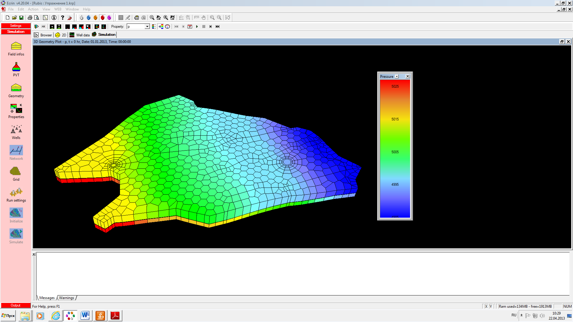
Fig. 13. Initial pressure field displayed in the 3d Geometry plot

Fig. 15. Initial saturations field displayed in the cross-section

Simulation: Run Simulation and Results Visualization

Run Simulation

After clicking on “Simulate” button simulation starts and results are displayed in real time as the run goes on.

Looking at well results

Evolution of pressure and rates simulated at each wells are shown at specific plots – “Gauges-P01” and “Gauges-I02” (Application 1). Displayed properties can be chosen by clicking “Edit displayed settings” button.

T

Fig. 16. Time of the water breaks through

he highest liquid rate which takes place for first 1000 hrs then decreases and becomes constant at 2700 STB/D after 7000 hrs. After 19700 hrs water breaks trough and liquid rate decreases (Application 1).

Looking at Field Results

On the 3D Geometry plot it is possible to see the initial pressure field and the last stored pressure field. Also on the “3D Geometry Plot Display” in the “Cross-Section” tab a horizontal cross-section at a desirable depth can be chosen.

I

Fig. 17. Final pressure field at 5960 ft

choose a depth 5960 ft and the last stored pressure (Fig. 17).

It is seen from the picture that the strongest pressure depletion is located near production well. And the higher pressure values are located in the north-west part where shale rock are crossed by the 5960ft horizontal cross-section.

On the 2D Geometry plot I can set a current stratigraphic depth and see evolution of selected properties with time (Fig. 18).

F

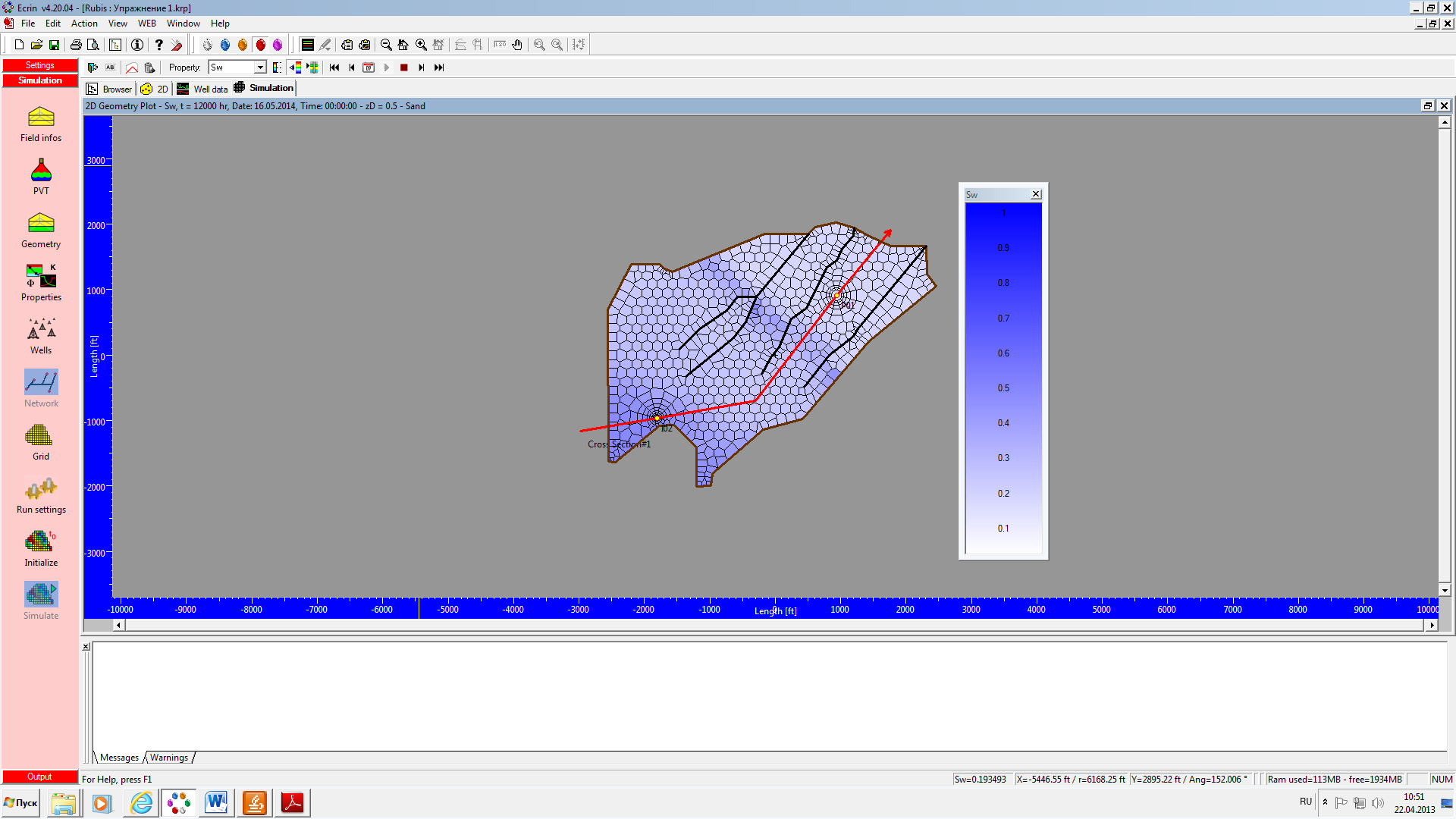
Fig. 18. Evolution of water saturation with time in the Sand Layer

inal saturation field show us that water invades the top layer by passing across the null-thickness region of the shale layer (Fig. 19).

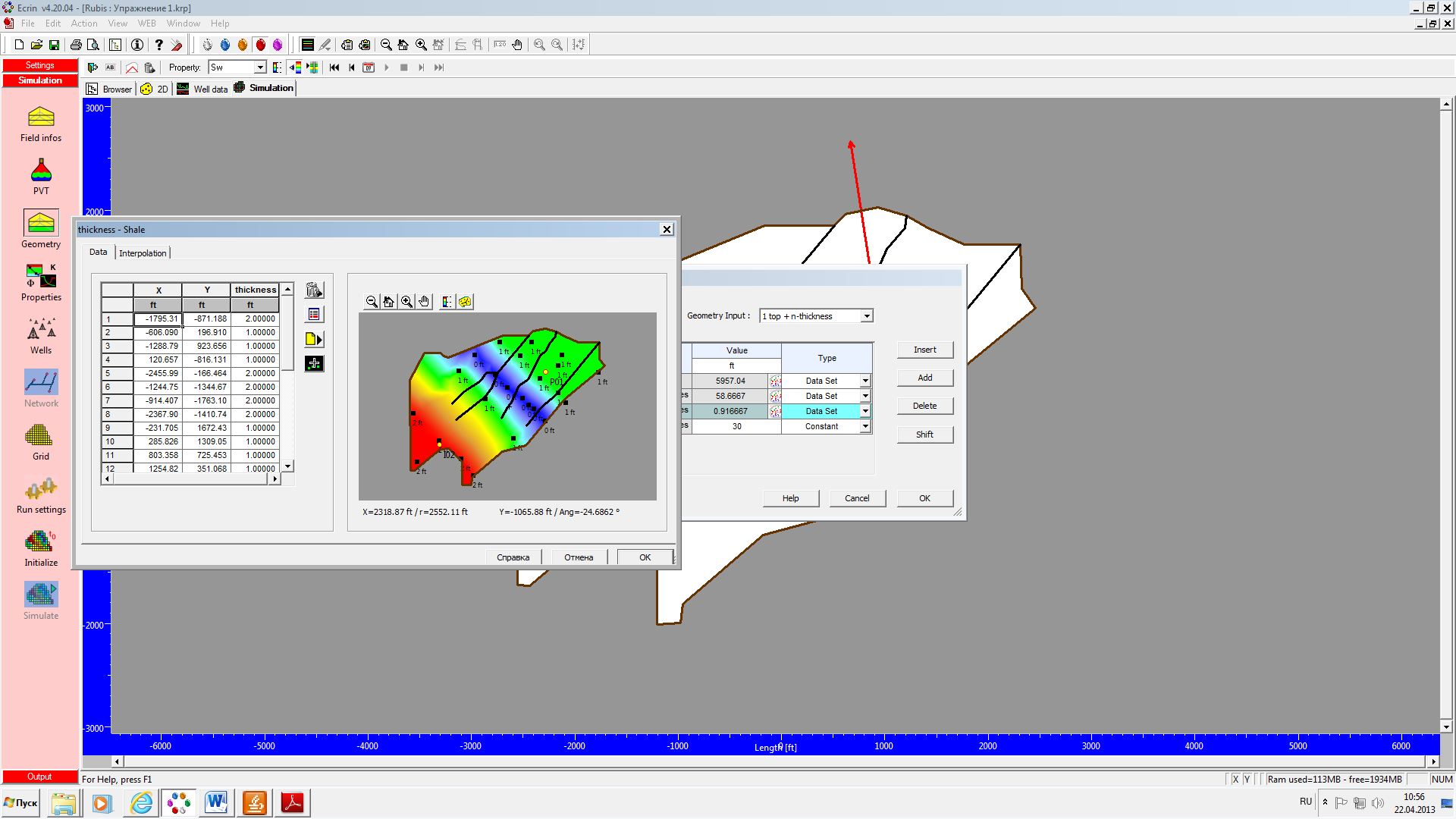
Fig. 19. Comparison of the shale thickness map (left) with the final S_w field in the Sand layer (right)

After replaying the simulation on the Cross-Section plot I can read the last saturation values (Fig. 20).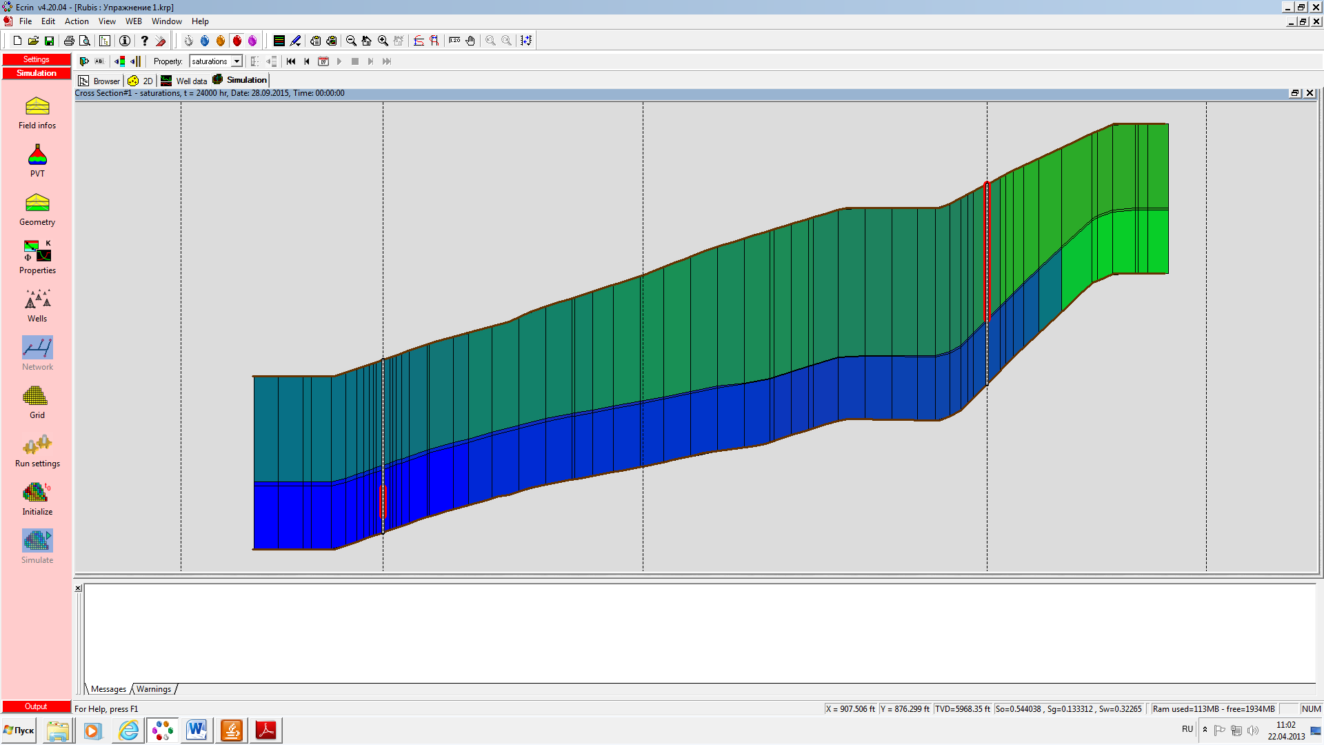

Fig. 20. S_o, S_g and S_w simulated in the vicinity of P01 after 1000 days of production

As can be seen above, some free gas appears by pressure depletion around P01 during the simulation (S_g=0.133312).

A pplication 1. Flow properties for P01