National Research Tomsk Polytechnic University

Petroleum learning centre

Rotaru Anna Vasilievna

Building an isothermal three-phase model in rubis

Report

Tomsk 2013

The aim of this course paper is to learn how to use Ecrin v4.20.04 for the purpose of building and simulation isothermal tree-phase model of oil field comprising two well – water injection and producer.

Rubis is chosen as an active model. Firstly, new project is created.

First part of work is made at the “2D Map” tab, which is displayed with several toolbars at the top.

Pvt Initialization

By clicking on “PVT” icon in the “Simulation” page the PVT definition is edited. Here I choose saturated oil with edition of water as the fluid type.

Model Construction: Defining the Reservoir Volumes Reservoir Lateral Definition: Contour and Faults

Clicking on the “Load Bitmap” icon I load the field bitmap from the file “RubGS01_FieldMap.bmp”. The map scale is indicated by using the “Scale” icon: I measured the distance which is on the map and enter the new distance in the Scale window.

T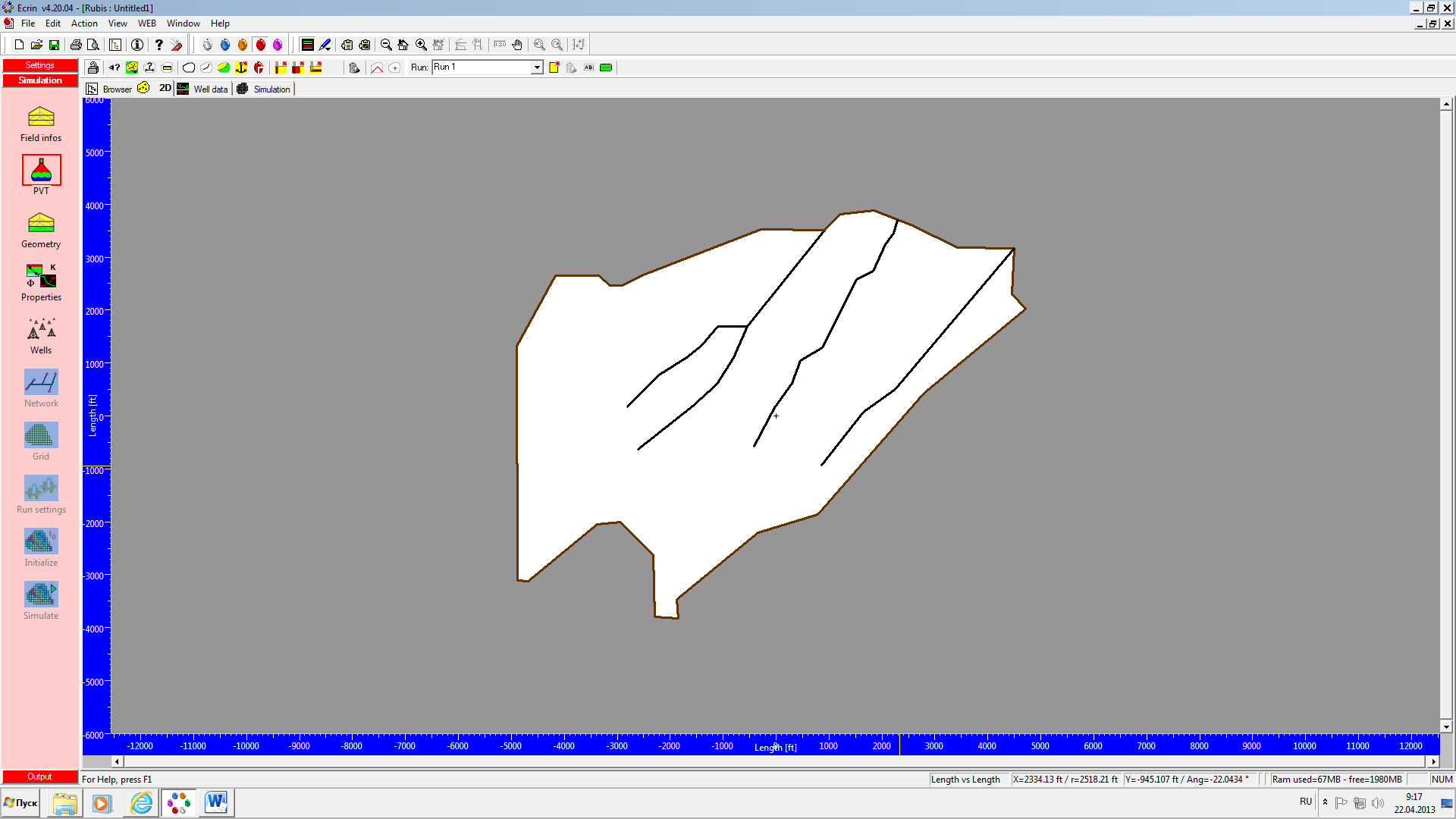 he contour of field and all faults are indicated by selecting the option “Draw contour” and “Create fault”. The current view of the reservoir can be chosen with the button “Edit display settings” (Fiq. 1).

Fig. 1. 2d Map after contour and faults creation Reservoir Vertical Definition: Defining the Layers

Using “Reservoir geometry” option in the “Simulation” page I define the reservoir structure: number and names of layers, top depth of reservoir and thickness of layers. There are 3 layers: sand, shale and bottom. Information about top surface and thickness of shale layers is loaded from the files “RubGS01_TopHorizon.asc” and “RubGS01_ShaleThickness.asc”, thickness of sand layers is entered by the hands using a special button (50 ft in the south-west of the reservoir, 40 ft in the north-east, with a maximum thickness of 70 ft in the center).

A First Preview of the Reservoir Geometry

A fter defining the layers it is able to build a vertical cross-section with the “Create cross-section” button. Changing location of red line I can see different cross-section and understand the dynamic of thickness changes (Fig. 12).

A

Fig. 2. Different cross-section

ccording to cross-section reservoir is a slope of anticline with layers dipping downward in south-west direction. Increasing of the sand layer depth takes place in the centre part of the reservoir.

Model Construction: Properties Definition

Defining Petrophysical Properties

Next step is to define petrophysical properties of layers.

Clicking on the “Properties” button in the “Simulation” page I open the “Reservoir – Properties” dialog, where desirable properties must be input. At first I choose “Layered” pattern of description on the top of window.

Then I create new properties set for sand and shale layers: sand rock and shale rock. Petrophisical properties for new set are contained in the left display.

After changing type of data from “Constant” to “Data Set” for sand rock I loaded information about its porosity and permability from files “RubGS01_SandPermeability.asc” and “RubGS01_SandPorosity.asc”.

The shale rock porosity, permability and leakage factor were chosen as constant properties: 0.001 mD, 0.05 and 0.05 accordingly.

The property set of bottom layers are default.