2.2. Impact of a tax on price and quantity

Without taxes – no government. Government is necessary for certain goods – known as “public goods” – to be efficiently provided. Taxes are needed to raise revenue to pay for public goods. Examples are Justice, Defense, Public Health Services, Roads, and Education. Taxes discourage market activity. When a good is taxed, the price paid by buyers increases and the quantity sold falls. A tax on a good places a wedge between the price paid by buyers and the price received by sellers. Buyers and sellers usually share the tax burden.

The incidence of a tax refers to who bears the burden of a tax. The incidence of a tax does not depend on who actually pays the tax to the government. The incidence of the tax depends on the relative price elasticities of supply and demand in the market.

To find out the impact of a tax on price and quantity we need to compute the new price under taxation. We can do it by changing supply function in proper way:

In the case of specific tax Q_s = c +dP should be transformed into Q_s^t = c +d(P-t).

In the case of Ad Valorem tax the original functions should be transformed into Q_s^t = c +d P (1-t).

Then we need to equal original (or constant) demand function and new (transformed) supply function to get the new characteristics of equilibrium P_e^t and Q_e^t.

Tax revenue (TaxR) is the whole sum of money collected by taxation. It can be computed as TaxR=t•Q_e^t.

The tax burden on consumers is the part of the tax paid by consumers in terms of higher prices. CB= (P_e^t - P_e)•Q_e^t.

The tax burden on sellers is the part of the tax paid by firms in terms of lower receipts. SB=TaxR – CB = t•Q_e^t - (P_e^t - P_e)•Q_e^t = Q_e^t (t - P_e^t + P_e)

Tax burden on each is determined by the elasticities of supply and demand.

Also we can define society tax burden – some losses of all the society because of decrease of quantity sold/bought on the market and increased price: SCB = t•( Q_e - Q_e^t).

In the case of subsidy government support supply curve shifts in opposite side and according to this action our calculation will change (Q_s^sub = c +d(P+sub)) and market actors get benefits instead of pay burden. But the main prinsiple remains the same.

Lecture 4. Elasticity and its applications

1. Demand elasticity

1.1. Price Elasticity Coefficient and Factors affecting price elasticity of demand

Arc-elasticity:

Point-elasticity:

Factors affecting price elasticity of demand:

Substitution - The more substitutes, the higher the elasticity, as people can easily switch from one good to another if a minor price change is made.

Percentage in the consumer’ income - The higher the percentage that the product's price is of the consumers income, the higher the elasticity, as people will be careful with purchasing the goods because of its cost.

Useful or not - The more necessary a goods is, the lower the elasticity, as people will buy it no matter the price, such as insulin.

The time period under consideration - The longer a price change holds, the higher the elasticity, as more and more people will stop demanding the goods (i.e. if you go to the supermarket and find that blueberries have doubled in price, you'll buy it because you need it this time, but next time you won't, unless the price drops back down again). Elasticity will normally be different in the short term and the long term.

Breadth of definition: The broader the definition, the lower the elasticity

Table of price elasticity kinds of demand

Demand	Coefficient	Illustration	Examples
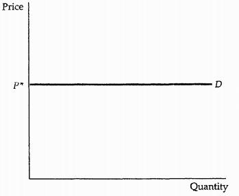
Infinitely (perfectly) elastic	|Edp|=∞		Diamands, goods on perfect competitive market
Elastic	|Edp|>1		Most goods in long term, also durable goods (automobile, TV set, frige etc.)
Unitary	|Edp|=1		Any good with the same reaction of both price and quantity demanded
Inelastic	0<|Edp|<1		Most goods in short term, also nondurable (food, services etc.)
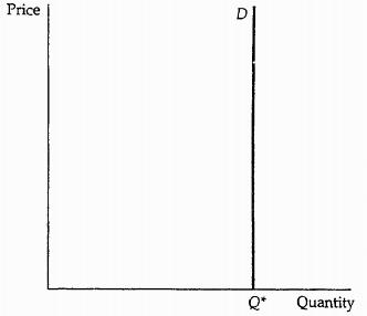
Completely Inelastic	|Edp| =0		Water, medicine for ill person, drugs for drug taker