

2. Results of MatLab code
2.1. Determining of the characteristics of the system
a. State space matrices of series connection “actuator+aircraft”:
sys =
a =
x1 x2 x3 x4 x5 x6 x7 x8
x1 0.0027 6.162 0 -9.801 0 0.0288 -0.2326 0
x2 -0.0011 -0.9623 1 -0.0026 0 0 -0.0636 0
x3 -0.0004 -5.692 -1.926 0.0013 0 0.0011 -3.45 0
x4 0 0 1 0 0 0 0 0
x5 0.0349 134.1 0 -134.1 0 0 0 0
x6 0 0 0 0 0 -0.6667 0 0.6667
x7 0 0 0 0 0 0 -10 0
x8 0 0 0 0 0 0 0 -10
b =
u1 u2
x1 0 0
x2 0 0
x3 0 0
x4 0 0
x5 0 0
x6 0 0
x7 10 0
x8 0 10
c =
x1 x2 x3 x4 x5 x6 x7 x8
y1 1 0 0 0 0 0 0 0
y2 0 1 0 0 0 0 0 0
y3 0 0 1 0 0 0 0 0
y4 0 0 0 1 0 0 0 0
y5 0 0 0 0 1 0 0 0
y6 0 0 0 0 0 1 0 0
d =
u1 u2
y1 0 0
y2 0 0
y3 0 0
y4 0 0
y5 0 0
y6 0 0
Continuous-time state-space model.
b. From 1st input
W1 =
-2.326 s^6 - 35.45 s^5 - 28.52 s^4 + 1291 s^3 + 3768 s^2 + 1937 s + 5.827e-22
------------------------------------------------------------------------------------
s^8 + 23.55 s^7 + 180.5 s^6 + 549.6 s^5 + 1047 s^4 + 501.2 s^3 + 4.875 s^2 + 3.841 s
Continuous-time transfer function.
W2 =
-0.636 s^6 - 42.5 s^5 - 385 s^4 - 236.4 s^3 - 2.658 s^2 - 2.465 s - 1.238e-24
------------------------------------------------------------------------------------
s^8 + 23.55 s^7 + 180.5 s^6 + 549.6 s^5 + 1047 s^4 + 501.2 s^3 + 4.875 s^2 + 3.841 s
Continuous-time transfer function.
W3 =
-34.5 s^6 - 397.5 s^5 - 544.7 s^4 - 198.3 s^3 - 1.107 s^2 - 7.284e-32 s
------------------------------------------------------------------------------------
s^8 + 23.55 s^7 + 180.5 s^6 + 549.6 s^5 + 1047 s^4 + 501.2 s^3 + 4.875 s^2 + 3.841 s
Continuous-time transfer function.
W4 =
-34.5 s^5 - 397.5 s^4 - 544.7 s^3 - 198.3 s^2 - 1.107 s + 7.746e-14
------------------------------------------------------------------------------------
s^8 + 23.55 s^7 + 180.5 s^6 + 549.6 s^5 + 1047 s^4 + 501.2 s^3 + 4.875 s^2 + 3.841 s
Continuous-time transfer function.
W5 =
-85.37 s^5 - 1075 s^4 + 1664 s^3 + 4.138e04 s^2 + 2.637e04 s - 114.5
------------------------------------------------------------------------------------
s^8 + 23.55 s^7 + 180.5 s^6 + 549.6 s^5 + 1047 s^4 + 501.2 s^3 + 4.875 s^2 + 3.841 s
Continuous-time transfer function.
W6 =0
Continuous-time transfer function.
From 2nd input
W1 =
0.192 s^5 + 2.475 s^4 + 6.968 s^3 + 14.15 s^2 - 0.7236 s - 4.938e-18
------------------------------------------------------------------------------------
s^8 + 23.55 s^7 + 180.5 s^6 + 549.6 s^5 + 1047 s^4 + 501.2 s^3 + 4.875 s^2 + 3.841 s
Continuous-time transfer function.
W2 =
0.007122 s^4 + 0.0707 s^3 - 0.005145 s^2 + 0.0007959 s - 1.155e-15
------------------------------------------------------------------------------------
s^8 + 23.55 s^7 + 180.5 s^6 + 549.6 s^5 + 1047 s^4 + 501.2 s^3 + 4.875 s^2 + 3.841 s
Continuous-time transfer function.
W3 =
0.007334 s^5 + 0.0803 s^4 + 0.07077 s^3 + 0.01159 s^2 - 2.967e-19 s + 1.068e-35
------------------------------------------------------------------------------------
s^8 + 23.55 s^7 + 180.5 s^6 + 549.6 s^5 + 1047 s^4 + 501.2 s^3 + 4.875 s^2 + 3.841 s
Continuous-time transfer function.
W4 =
0.007334 s^4 + 0.0803 s^3 + 0.07077 s^2 + 0.01159 s + 3.019e-16
------------------------------------------------------------------------------------
s^8 + 23.55 s^7 + 180.5 s^6 + 549.6 s^5 + 1047 s^4 + 501.2 s^3 + 4.875 s^2 + 3.841 s
Continuous-time transfer function.
W5 =
0.006701 s^4 + 0.05804 s^3 - 1.044 s^2 - 9.686 s - 1.473
------------------------------------------------------------------------------------
s^8 + 23.55 s^7 + 180.5 s^6 + 549.6 s^5 + 1047 s^4 + 501.2 s^3 + 4.875 s^2 + 3.841 s
Continuous-time transfer function.
W6 =
6.667 s^6 + 85.91 s^5 + 242.7 s^4 + 502.7 s^3 - 1.271 s^2 + 3.841 s + 2.62e-19
------------------------------------------------------------------------------------
s^8 + 23.55 s^7 + 180.5 s^6 + 549.6 s^5 + 1047 s^4 + 501.2 s^3 + 4.875 s^2 + 3.841 s
Continuous-time transfer function.
c. Frequency responses (Bode and Nyquist) of this connection from all inputs to
n-th output:
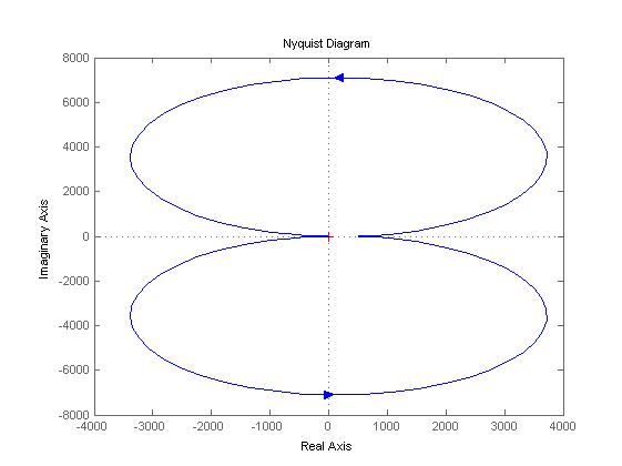
Fig.1. Nyquist plot from 1st input to 1st output
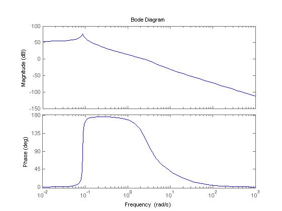
Fig.2.Bode plot from 1st input to 1st output
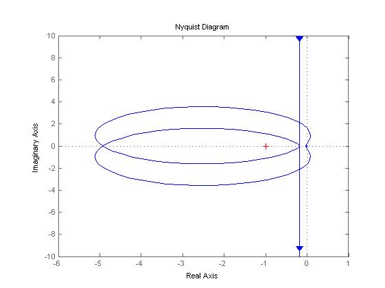
Fig.3.Nyquist plot from 2nd input to 1st output
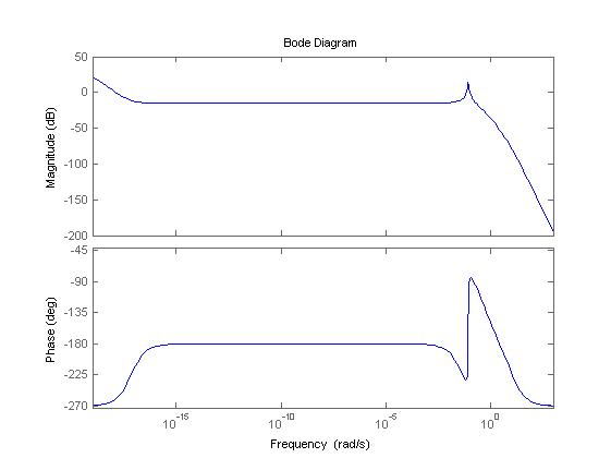
Fig.4.Bode plot from 2nd input to 1st output
d. Eigenvalues of state matrix of the open-loop system
Eol = 0
-1.4459 + 2.3372i
-1.4459 - 2.3372i
0.0031 + 0.0873i
0.0031 - 0.0873i
-0.6667
-10.0000
-10.0000
e. Graphic representation of these eigenvalues on the complex plane

Fig.5. Graphic representation of eigenvalues on the complex plane
f. Eigenvalues of state matrix of the closed-loop system
Ecl = -11.9151
3.1030 + 2.3874i
3.1030 - 2.3874i
-3.5884 + 3.2216i
-3.5884 - 3.2216i
0.0041
-0.6707
-10.0000
g. Graphic representation of the eigenvalues of the received closed-loop system on the complex plane
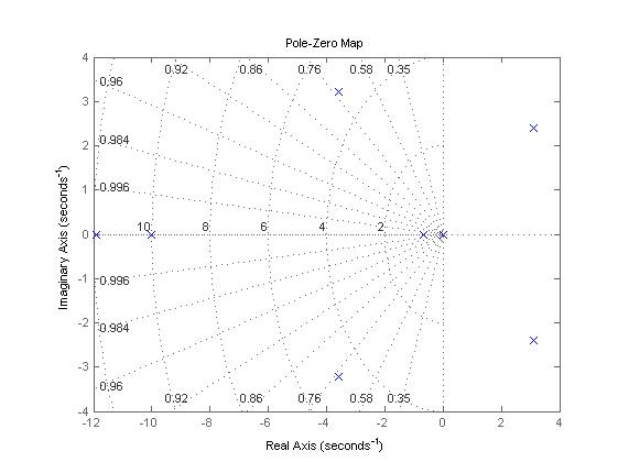
Fig.6. Graphic representation of the eigenvalues of the received closed-loop system on the complex plane
h. H2-norm for the closed-loop system:
The "gram" command cannot be used for models with unstable dynamics.
i. H∞-norm for the closed-loop system:
Hinf = 11.8700