1.
The important aspect in control systems engineering is stability of systems. It should be provided in all cases of system usage.
Let’s consider the problem of improvement of system dynamic properties with the help of feedback.
1st stage. Let’s consider linear system described by the differential equation
![]()
Where x is a state vector of system, u is a control vector, A is a state matrix of system, which dimension is equal to nxn, B is a control matrix of system, which dimension is equal to lxn.
At the first stage of synthesis of the optimal deterministic controller it is necessary to set four matrices [A, B, C, D], which describe system in the state space, where the size of matrix C coincide with the size of matrix A. that is l=n.
Matrix D in the most cases is zero matrix.
The controller is necessary to synthesize for series connection of actuator and plant as dynamics of steering devices and aircraft motion is described by separate equations set.
2nd stage. Let us solve a problem of construction of the optimal deterministic controller which minimizes quadratic integral criterion
![]()
where
R1,
R2,
P1
are positively defined symmetric matrices. R1=CTR3C,
where R3
is positively defined symmetric matrix. The first component ![]() is a measure of deviation from zero state of system at the moment of
time t.
is a measure of deviation from zero state of system at the moment of
time t.
The second term of criterion takes into account power costs for control.
The
terminal component ![]() is included in criterion if it is necessary to ensure the maximal
closeness of a terminal state x (t1)
to zero value.
is included in criterion if it is necessary to ensure the maximal
closeness of a terminal state x (t1)
to zero value.
The square root of this equation refers to as H2-norm.
As the case when parameters of system are constant, i.e. A, B, C, R1, R2 are constant is considered so it is possible to present the quadratic integral criterion as
![]()
To minimize the criterion it is necessary to solve Ricatti equation.
![]()
For this equation we shall receive the following control law
![]()
where
![]()
Thus, at the second stage of synthesis the quadratic integral performance index is minimized. For this purpose the weight factors R1 and R2, which take into account value of each parameters at state and control, are set, and algebraic Ricatti equation is solved.
As the result of synthesis we receive the controller as coefficients of F at which the performance index will have the minimal value.
In Matlab software it is possible to construct the optimal deterministic controller, using operator lqr:
[F, P, E]= lqr(A,B,R1,R2)
As it is easy to see, to solve this problem it is necessary to set weight matrices R1, R2 and matrices of control plant (A,B).After performance of this operator it is received:
-matrix F is matrix of optimal gains of controller;
-matrix P which is the solution of Ricatti equation
-vector E that contains eigenvalues of state matrix of closed loop system A-BF.
In Matlab software it is possible to calculate the performance index, using the operator normh2:
H2=normh2(A0,B0,C0,D0).
2.
BRIEF THEORETICAL INFORMATION
Let us consider the improvement problem of dynamic properties of a discrete control system with the help of feedback.
1st stage. We shall consider a linear discrete system which is described by the differential equation
x(i+1) = A(i)x(i) + B(i)u(i),
where x is a state vector of system, A is a state matrix of system, which dimension is equal to nxn, B is a control matrix of system, which dimension is equal to n x m.
The control variable is described by the equation
y(i) = C(i)x(i),
where y is a vector of the measured variables (observation vector), C is a observation matrix, which dimension is equal to l x n.
Let us assume that all variables are measured, that is the full state x of control plane can be measured accurately at any moment of time and used for creation of feedback.
Thus, at the first stage of synthesis of the optimal deterministic discrete controller it is necessary to set the four of matrices {A,B,C,D}, which describe a system in state space, where the size of matrix C should coincide with the size of matrix A, that is l = n.
Matrix D in the most cases is zero matrix.
As well as in a continuous case, the controller is necessary to synthesize for series connection of actuator and plant as dynamics of steering devices and aircraft motion is described by separate equations set.
2nd stage. Let us solve a problem of construction of the optimal deterministic discrete controller which minimizes quadratic integral criterion
![]() (2.2.1)
(2.2.1)
Here the control law is described by the equation
u(i) = -Fx(i) (2.2.2)
To minimize the criterion (2.2.1) it is necessary to solve discrete Riccati equation.
![]()
E = eig(A-BF)
Thus, at the second stage of synthesis the quadratic integral performance index (2.2.1) is minimized. As a result of synthesis we receive a controller as elements of matrix F (2.2.2), at which the performance index (2.2.1) will have the minimum.
In MatLab software it is possible to construct the optimal deterministic discrete controller, using the operator dlqr:
[F, S, E] = dlq (A, B, R1, R2)
As it is easy to see, to solve this problem it is necessary to set weight matrices R1, R2 and matrices of control plant (A, B).
After performance of this operator it is received:
matrix F is matrix of optimal gains of discrete controller;
matrix S which is the solution of discrete Riccati equation;
vector E that contains eigenvalues of a state matrix of closed loop system A-BF.
This operator can be used if it is given the discrete plant and it is necessary to receive a discrete controller.
The operator lqrd is necessary to be used if it is given the continuous plant and it is necessary to receive a discrete controller.
In MatLab software it is possible to construct the optimal deterministic discrete controller, using the operator dlqr:
[F, S, E] = dlq (A, B, R1, R2, Ts),
where Ts is sampling time.
This problem can be solved according with the following algorithm:
The continuous plant (A, B, C, D) and continuous weight matrices (R1, R2) is sampled with the help of the zero order hold with sampling time Ts.
Matrix of optimal gains F of a discrete controller is calculated.
As at calculation of H2-norm of the deterministic discrete system it is used controllability gramian Gd of the closed loop system which can be found from the solution of the discrete Lyapunov equation:
AclGdATcl – Gd + BclBTcl = 0
The square of H2-norm for the deterministic case can be received as follows:
J2d = trace(Cw0Gd(Cw0)T)
where Cw0 is a weight matrix of observation:
Cw0 = CclQ; Q = diag(q1…..qn),
where q1…..qn are weight coefficients of state space variables.
In MatLab software it is possible to calculate a performance index for discrete systems, using the following algorithm:
BB=Bcl*Bcl ‘;
G=dlyap (Acl, BB);
H2d=trace (Ccl*G*Ccl ‘)
With the help of the operator dlyap we shall receive the solution of the discrete Lyapunov equation, the operator trace determines the trace of matrix.
3.
For continuous:
To set four matrices [A1,B1,C1,D1] described the aircraft dynamics and [A2,B2,C2,D2] described the actuator dynamics.
To present the model of aircraft dynamics and the model of actuator dynamics in state space with the help of the operator ss.
To make series connection of the model of actuator dynamics and the model of aircraft dynamics with the help of the operator series.
To extract four of matrices [A,B,C,D] of the received connection with the help of the operator ssdata.
As a dimension of the system has increased by 1 parameter, therefore it is necessary to extend the observation matrix of the system:
C3=[C;zeros(1,5) ]; D3=zeros(6,1);
sysser1=ss(A,B,C3,D3);
W=[0.01 1 3 1.5 1 0.5];
R1=diag(W);
R2=0.5;
[F,P,E]=lqr(A,B,R1,R2)
To close the model of system described in state space [A,B,C3,D3] by the synthesis controller with the help of the operator feedback.
To calculate the PI with the help of operator normh2.To build the step response of the received closed loop system with the help of the operator step.
To calculate the PI of uncompensated system(without controller) and compare the values of PI of uncompensated and compensated systems.
For discrete:
To set four matrices [A1,B1,C1,D1] described the aircraft dynamics and [A2,B2,C2,D2] described the actuator dynamics.
To present the model of aircraft dynamics and the model of actuator dynamics in state space with the help of the operator ss.
To make series connection of the model of actuator dynamics and the model of aircraft dynamics with the help of the operator series.
To make the conversion from continuous description to discrete one with the help of the operator c2d with sampling time 0.01 sec.
To extract four of matrices [A,B,C,D] of the received connection with the help of the operator ssdata.
To extract four matrices [Ad,Bd,Cd,Dd] of the received connection with the help of the operator ssdata for discrete case.
As a dimension of the system has increased by 1 parameter, therefore it is necessary to extend the observation matrix of the system:
C3=[C;zeros(1,5) ]; D3=zeros(6,1);
sysser1=ss(A,B,C3,D3); %for continuous model
sysser1d=ss(Ad,Bd,C3,D3); %for discrete model
To synthesize the optimal deterministic discrete controller, using the operator dlqr. For this purpose it is necessary to set a diagonal matrices of weight factors Q and R.
W=[0.01 1 3 1.5 1 0.5];
R1=diag(W);
R2=0.5;
[F,P,E]=lqr(Ad,Bd,R1,R2)
To close the discrete plant (sysser1d) by the synthesized controller with the help of the operator feedback.
Calculate the PI with the help of the operators dlyap, trace.
Construct the optimal deterministic discrete controller, using the operator lqrd for the given continuous plant.
Close continuous plant(sysser1) by the synthesized discrete controller with the help of the operator feedback.
Calculate a PI with the help of the operator normh2.
4) Conception of linear dynamic system observer. Kalman filter. (Continuous case)
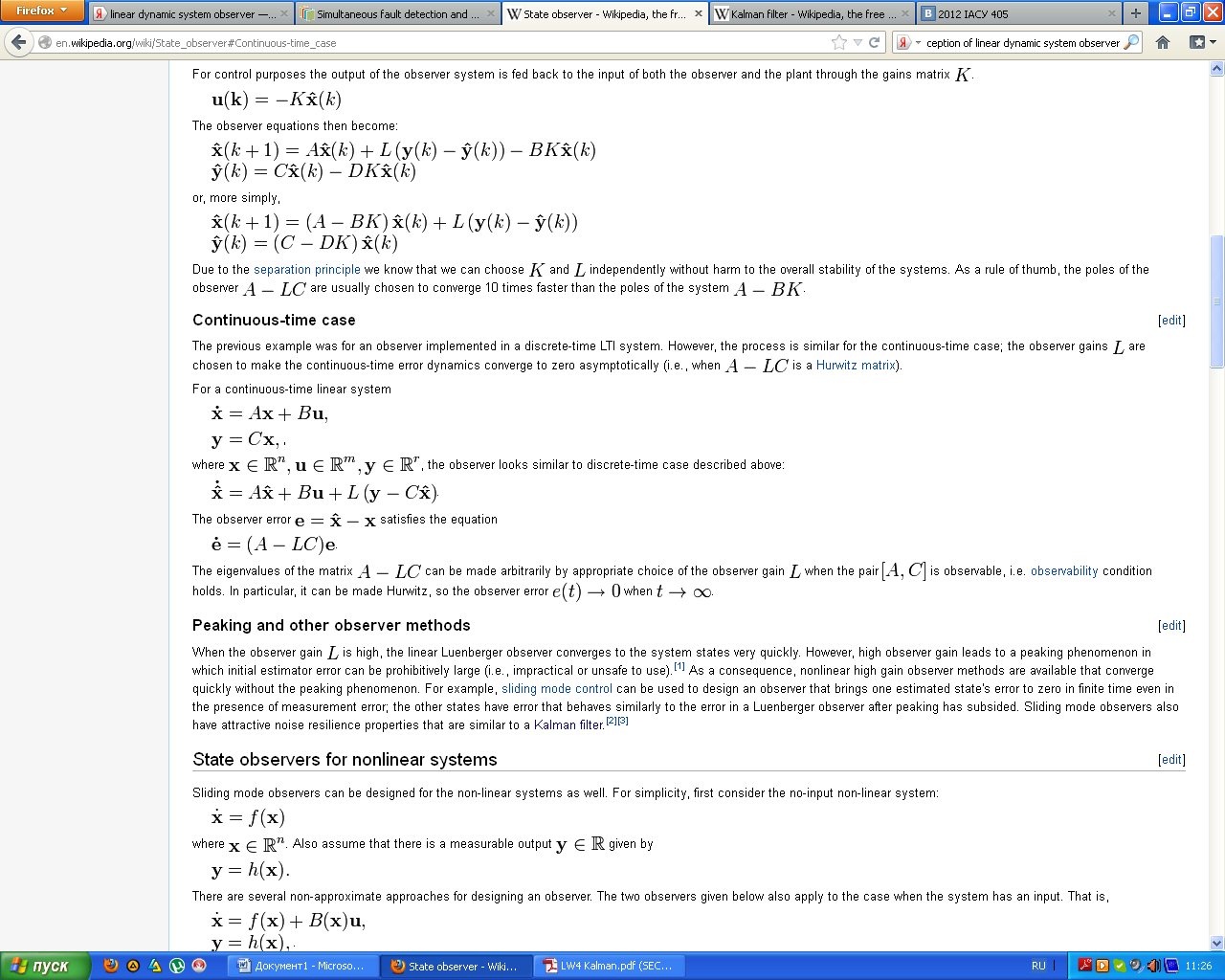
In control theory, a state observer is a system that provides an estimate of the internal state of a given real system, from measurements of the input and output of the real system. It is typically computer-implemented, and provides the basis of many practical applications.
Knowing the system state is necessary to solve many control theory problems; for example, stabilizing a system using state feedback. In most practical cases, the physical state of the system cannot be determined by direct observation. Instead, indirect effects of the internal state are observed by way of the system outputs. A simple example is that of vehicles in a tunnel: the rates and velocities at which vehicles enter and leave the tunnel can be observed directly, but the exact state inside the tunnel can only be estimated. If a system is observable, it is possible to fully reconstruct the system state from its output measurements using the state observer.
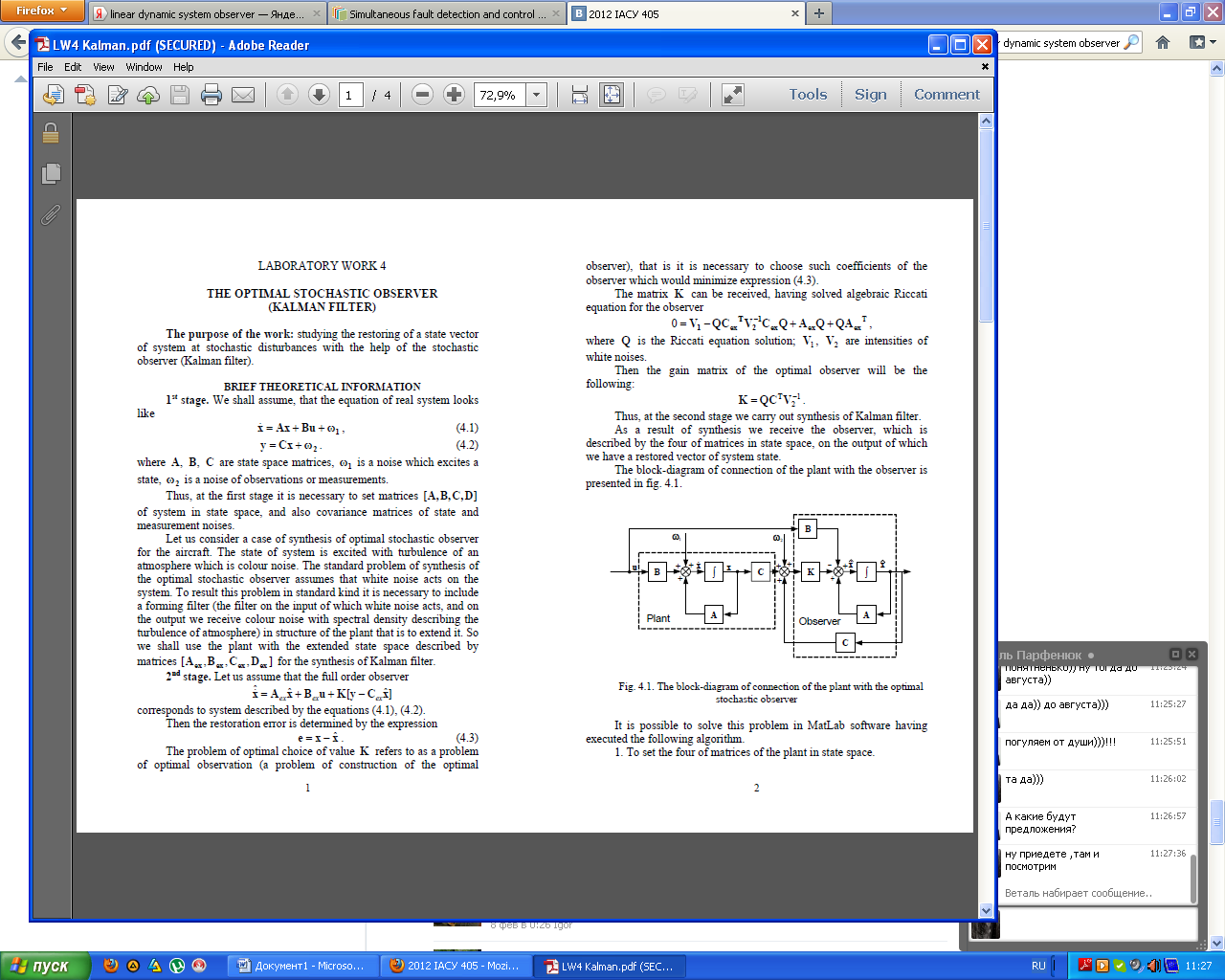
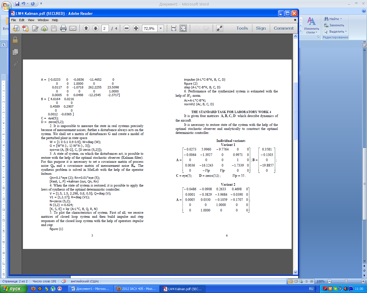
5) Kalman filter. Solution of problem on analytical desisgning of optimal observers with the help of computer. (Continuous case)
6)
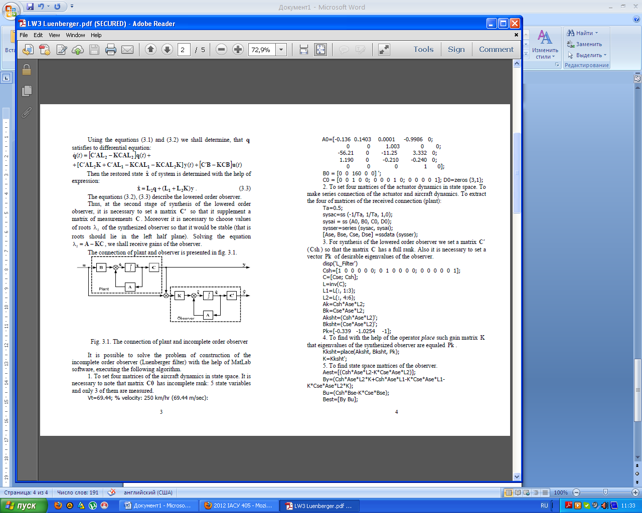
Reduced order observers. Luenberger filter.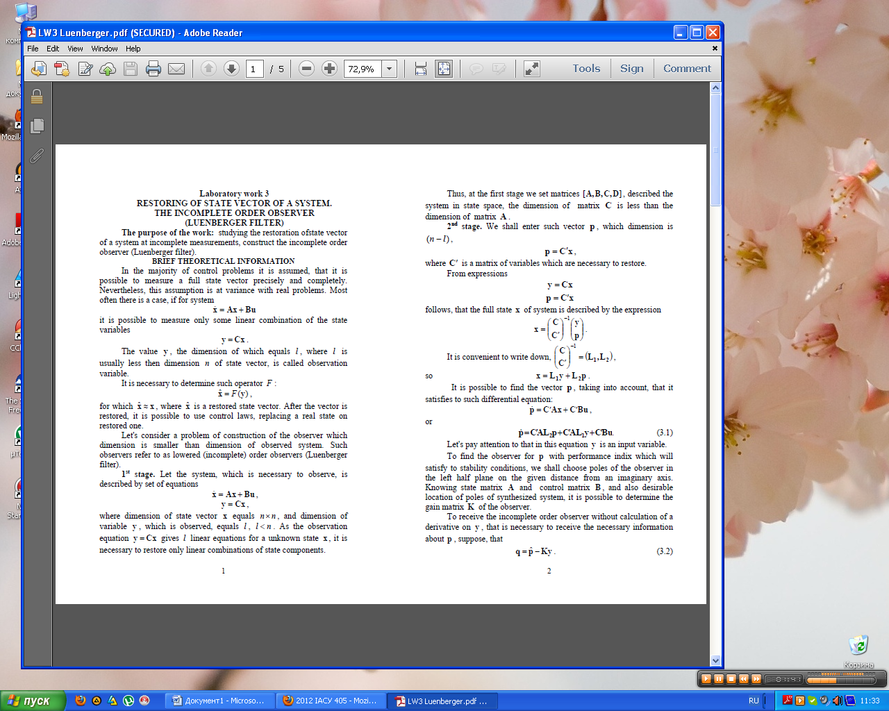
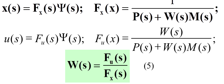
7. Synthesis of optimal control systems in frequency domain. Performance index for stochastic systems.
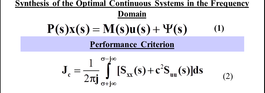
And the transfer function is as follows:
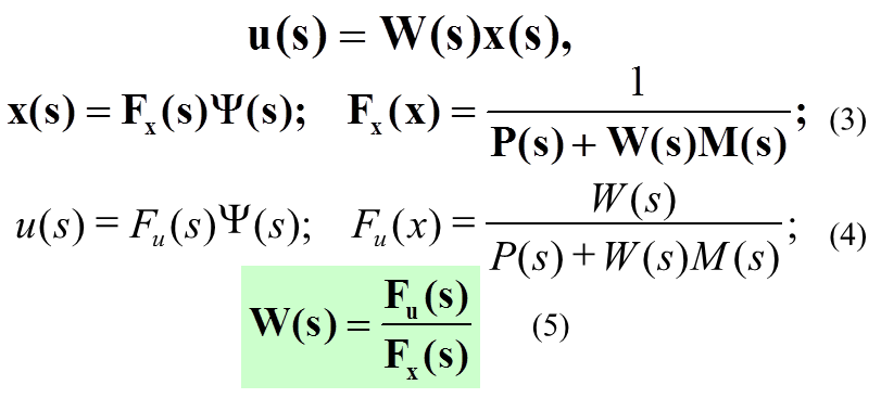
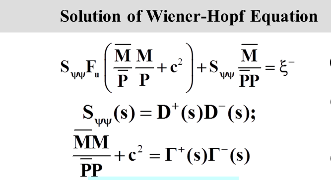
8. Wiener-Hopf equation… and transfer function…
The Wiener–Hopf method was initially developed by Norbert Wiener and Eberhard Hopf as a method to solve systems ofintegral equations, but has found wider use in solving two-dimensional partial differential equations with mixed boundary conditions on the same boundary. In general, the method works by exploiting the complex-analytical properties of transformed functions. Typically, the standard Fourier transform is used, but examples exist using other transforms, such as the Mellin transform.

tf: