Properties

Properties of the z-transform
	Time domain	Z-domain	Proof	ROC
Notation				ROC:
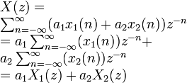
Linearity				At least the intersection of ROC1 and ROC2
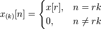
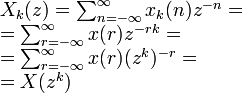
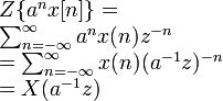
Time expansion	: integer			R^{1/k}
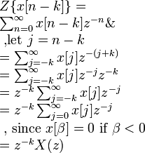
Time shifting				ROC, except if and if
Scaling in the z-domain
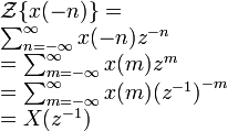
Time reversal
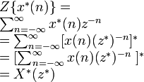
Complex conjugation				ROC
Real part				ROC
Imaginary part				ROC
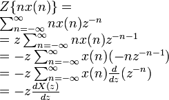
Differentiation				ROC
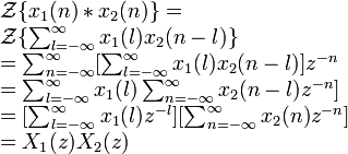
Convolution				At least the intersection of ROC1 and ROC2
Cross-correlation				At least the intersection of ROC of and
First difference				At least the intersection of ROC of X1(z) and
Accumulation
Multiplication				-
Parseval's relation

• Initial value theorem

, If causal

• Final value theorem

, Only if poles of are inside the unit circle

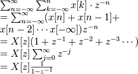
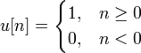
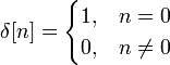
Table of common z-transform pairs

Here:

• 

• 

	Signal,	Z-transform,	ROC
1
2
3
4
5
6
7
8
9
10
11
12
13
14
15
16
17
18
19
20
21

Relationship to Laplace transform

The Bilinear transform is a useful approximation for converting continuous time filters (represented in Laplace space) into discrete time filters (represented in z space), and vice versa. To do this, you can use the following substitutions in H(s) or H(z):

from Laplace to z (Tustin transformation), or

from z to Laplace. Through the bilinear transformation, the complex s-plane (of the Laplace transform) is mapped to the complex z-plane (of the z-transform). While this mapping is (necessarily) nonlinear, it is useful in that it maps the entire axis of the s-plane onto the unit circle in the z-plane. As such, the Fourier transform (which is the Laplace transform evaluated on the axis) becomes the discrete-time Fourier transform. This assumes that the Fourier transform exists; i.e., that the axis is in the region of convergence of the Laplace transform.