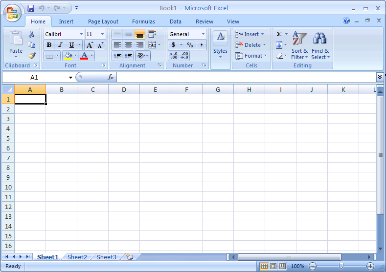
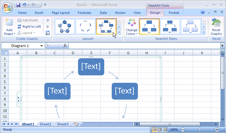
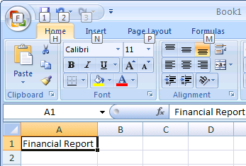
Becoming Familiar With The Excel 2007 Screen
Becoming
familiar with the Microsoft Excel new user interface is very
important in order for you to learn the program effectively. This
lesson describes the screen elements in Excel 2007 in detail. Some
of the screen elements can be “toggled” on or off. For this
lesson, you screen may look slightly different to the illustration
below due to your own settings.
Office
Button
Quick
Access
Toolbar
Ribbon
Dialog
Box Launcher
Tabs
Help
Button
Title
Bar


Name
Box
Formula
Bar
Row
Heading
Column
Heading
Active
Cell


Sheet
Tab


Vertical Scroll Bar
Horizontal
Scroll Bar


Status
Bar
View Buttons
Zoom
Controls
Screen Elements
|
Functions
|
Office Button
|
Replaces
the File menu available in earlier versions of Microsoft Office
and contains the same basic commands to open, save, and print.
However, in the 2007 Office release, more commands are now
available, such as Finish and Publish.
|
Quick
Access Toolbar
|
A
customizable toolbar that contains a set of commands that is
independent of the tab that is currently displayed.
|
Title Bar
|
Displays
the program name and the workbook name you are working on.
|
Tabs
|
Display
the commands that are most relevant for each of the task areas in
the applications.
|
Help Button
|
Displays
the Excel Help window.
|
Name Box
|
Shows
the selected cell, drawing object or chart item. You can also use
it to name a selected cell / range or move to the selected cell /
range.
|
Formula Bar
|
Displays the content (value
or formula) of the active cell. You can also edit the formula
here.
|
Active Cell
|
The selected cell in which
data is entered when you begin typing. Only one cell is active at
a time. The active cell is bounded by a heavy border.
|
Column Heading
|
Shows the column reference
letter.
|
Row Heading
|
Shows the row reference
number.
|
Sheet Tab
|
Shows the sheet name.
|
Horizontal Scroll Bar or
Vertical Scroll Bar
|
Help you to scroll through
your worksheet using the mouse.
|
Status Bar
|
Displays information about a
selected command or an operation in progress. The right side of
the status bar shows whether the keys (CAPS LOCK, SCROLL LOCK, or
NUM LOCK) are turned on.
|
Contextual
Tab
Appears
in the interface only when they are useful for the type of task you
are currently performing
Options
Galleries
Display
available options quickly


Live
Preview
A
new feature that shows a preview of how an option affects the
selected object/element when you hover over different choices. It
helps you to preview the effects before committing to the options.
Using
the Excel 2007 Ribbon
The
traditional menus and toolbars have been replaced by the Ribbon —
a new device that presents commands organized into a set of tabs. The
tabs on the Ribbon display the commands that are most relevant for
each of the task areas in the applications. Office Excel 2007
provides three types of tabs on the Ribbon: Standard
tab,
Contextual
tab
and Program
tab.
Three
types of Tabs on the Ribbon
|
|
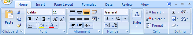
Standard
tab
|
The
standard set of tabs that you see on the Ribbon whenever you
start Excel 2007: Home, Insert, Page Layout, Formulas, Data,
Review, and View.
|
|
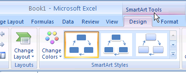
Contextual
tab
|
Contextual
tab appears in the interface only when they are useful for the
type of task you are currently performing, for example Drawing
Tools, SmartArt Tools or Table.
|
|
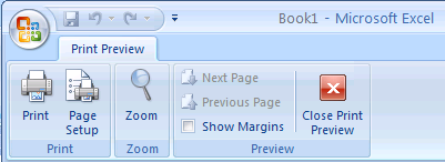
Program
tab
|
Program
tabs replace the standard set of tabs when you switch to certain
authoring modes or views, such as Print Preview, as shown below.
|
|
How To Work With The Ribbon
SUMMARY
Click
the tab you want.
Click
the command button or the option you want from the Ribbon.
|
TIPS
|
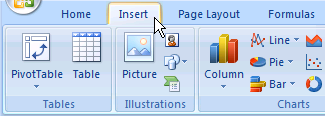
Click the Insert
tab.
The
Ribbon consists of tabs that are organized around specific
scenarios or objects. The controls on each tab are further
organized into several groups, for example Tables, Illustrations
and Charts, as shown below. The Ribbon can host richer content
than menus and toolbars can, including buttons, galleries, and
dialog box content.
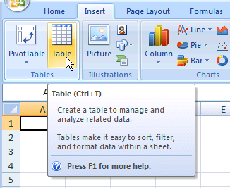
Click
the button and then click a command or option.
Command
buttons in each group carry out a command or display a menu of
commands. You can also click the button arrow to access lists
and galleries.
|
How To Use The Contextual Tabs
SUMMARY
Select
the object you want to change.
Click
the contextual tab.
Click
the command button you want.
|
|
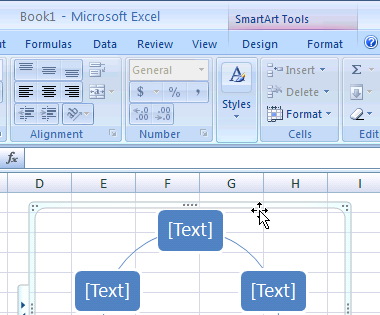
Select the object you
want to work with.
The
name of the applicable contextual tab, such as the SmartArt
Tools tab appears in an accent color, as shown below:
Click
the contextual tab.
The
contextual tab displays controls for the selected object.
Click
the command button you want.
You
can also click the button arrow to access lists and galleries.
|
How To Use the Dialog Box Launchers
SUMMARY
Click
the
 Dialog Box Launchers.
Select
the command or the option you want.
Click
the OK button or
the Close button.
|
|
Dialog Box Launchers are
small icons that appear in some groups. Clicking a Dialog Box
Launcher opens a related dialog box or task pane. In this
example, we will open the Format Cells dialog box.
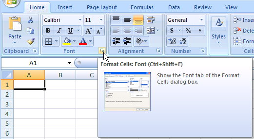
Click the Home
tab. Move your mouse pointer over the Font
Dialog Box Launchers.
A
ScreenTip with a thumbnail of the dialog box appears to show you
the dialog box it opens, as shown below.
Click
the Dialog Box Launchers.
The
Format Cells dialog box appears, as shown below.
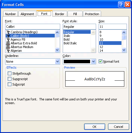
Select
an option and then click the OK
button.
The
dialog box closes.
|
How To Use Live Preview
SUMMARY
Select
the object you want to change.
Move
your mouse pointer over the option to preview the changes of
the object.
|
TIPS
|
Live
Preview temporarily applies the formatting on the selected text
or object, when you move your mouse over a formatting
button/option. The temporary formatting disappears when the
mouse pointer is moving away from it. This allows the users to
preview the effects without actually applying it on the selected
text or object. In this example, we will show you how to view or
apply a new style on a SmartArt.
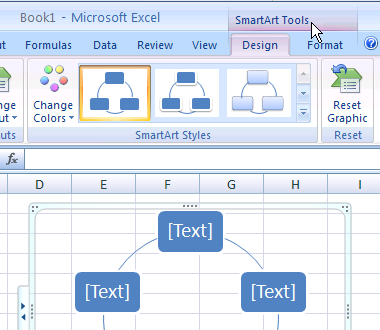
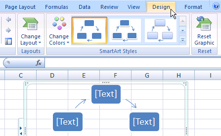
Select the SmartArt
you want to work with. Click the Design
tab.
Excel
2007 displays SmartArt Styles options in the Ribbon, as shown
below.
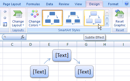
M ove
the mouse pointer over the Subtle
Effect style on the SmartArt
Styles group.
The
new style temporarily applies to the selected SmartArt, as shown
below. You can click the scroll up or scroll down arrow for more
styles. Alternatively, you can click the More list arrow
ove
the mouse pointer over the Subtle
Effect style on the SmartArt
Styles group.
The
new style temporarily applies to the selected SmartArt, as shown
below. You can click the scroll up or scroll down arrow for more
styles. Alternatively, you can click the More list arrow
 to enlarge the style box to show more styles.
|
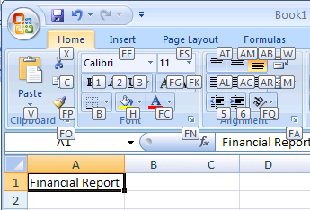
How To Use Access Keys
SUMMARY
Press
<Alt> key.
Press
the key as shown in the KeyTips.
|
TIPS
To
cancel the action that you are taking and hide the KeyTips,
press and release the <ALT> key again.
To
minimize or restore the Ribbon, press <CTRL>+<F1>.
|
|
If
you prefer to access the Ribbon using the keyboard or your mouse
is having a problem, you can use keyboard shortcuts to quickly
perform tasks without reaching for the mouse.
Press <Alt>.
The
KeyTips are displayed over each feature that is available in the
current view. You can also press <F10> instead of <Alt>.
To cancel the access keys, press either of these keys again.
Press
<H>.
The
KeyTips are displayed over each button in the current Ribbon.
Press
<1> to bold the
selected text.
The
selected text is bold, as shown below.

|
Working
with the Office Button And Toolbars
The
Office
Button,
located on the upper-left corner of the Excel window, replaces the
File menu and provides access to common functionality across all
Office applications, including Opening, Saving, Printing, and Sharing
a file.
The
Quick
Access Toolbar
is located by default at the top of the Excel window and provides
quick access to tools that you use frequently.
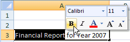
Mini
toolbar
pops up near the selected text whenever some text is selected. It
provides quick access to some common formatting toolbar buttons, such
as font, font size, bold, italic, font color, increase font size and
decrease font size. When the mouse pointer is moved away from it,
the toolbar becomes semi-transparent to allow an almost unobstructed
view of what's beneath. But when the mouse pointer moves over it, it
becomes opaque and ready for use.
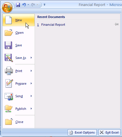
How To Use The Office Button
SUMMARY
Click
the Office Button.
Click
the command you want.
|
TIPS
|
Move the mouse pointer
over the Office Button.
Excel
2007 displays a ScreenTip to show a brief description of the
button.
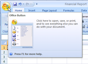
Click
the Office Button.
Excel
2007 opens the menu, as shown below.
Click
New.
The
New Workbook dialog box appears. You can use a shortcut key to
choose a command. In this example, press <Ctrl>+<N>.
This will create a new default workbook.
|
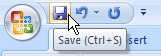
How To Use the Quick Access Toolbar
SUMMARY
On
the Quick Access Toolbar,
click the button, or the list arrow.
Click
the command or the option you want.
|
|
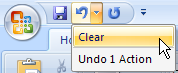
Move the mouse pointer
over the Save
button on the Quick Access Toolbar.
Excel
2007 displays a ScreenTip to show a brief description of the
button, as shown below.
Click
the button, or list arrow, and then click a command or
option.
By
default, the Quick Access Toolbar contains buttons for Save,
Undo and Redo. You may customize the toolbar by adding icons for
New, Open, Print, Print Preview, and etc.
|
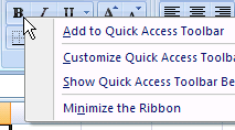
How To Add a Command To The Quick Access Toolbar
SUMMARY
On
the Quick Access Toolbar,
click the Customize Quick
Access Toolbar list arrow.
Click
the command you want to add to the Quick Access Toolbar.
|
TIPS
|
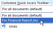
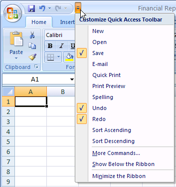
Click the Customize
Quick Access Toolbar list arrow.
A
pull-down menu appears, as shown below:
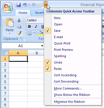
Click
the command you want to add to the Quick Access toolbar.
The
checked items appear on the toolbar.
|
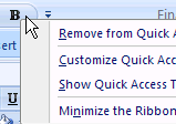
How To Remove A Command From the Quick Access Toolbar
TIPS
|
Click the Customize
Quick Access Toolbar list arrow, and then click
a button name.
The
unchecked item is removed from the toolbar.
|
How To Customize the Quick Access Toolbar
SUMMARY
Click
the Customize Quick Access Toolbar
list arrow and then click More
Commands.
Click
the Choose commands from
list arrow, and then select a specific Ribbon.
In
the left list box, click the command you want to add, and then
click the Add
button.
Click
the OK button.
|
TIPS
If
you want the commands available only in this workbook, select
the current workbook from the Customize Quick Access Toolbar
list box.
|
|
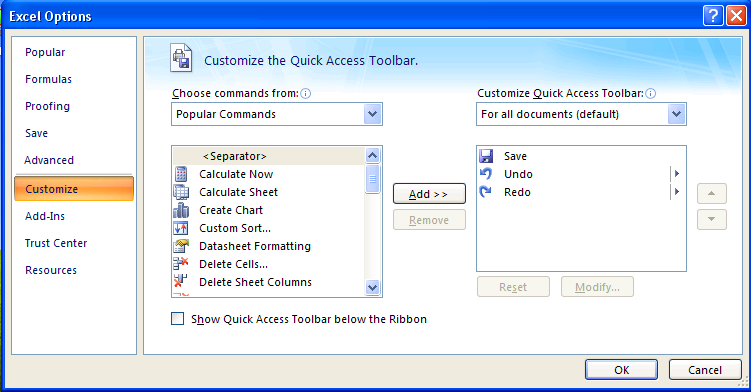
Click the Customize
Quick Access Toolbar list arrow, and then click
More Commands.
Excel
Options dialog box appears, the Customize option is selected by
default, as shown below:
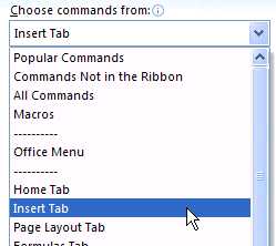
Click
the Choose commands from
list arrow, and then select the Ribbon where the button is
located.
All
commands under the selected Ribbon appear in the left list box
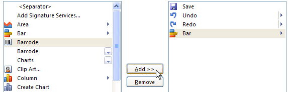
In
the left list box, click the command you want to add, and then
click the Add
button.
The
selected item is added to the list box on the right, as shown
below. You can click the Move Up and Move Down arrow buttons to
rearrange the order.
Click
the OK
button.
The
Excel options dialog box closes and the selected items are added
to the Quick Access Toolbar.
|
How To Move the Quick Access Toolbar
SUMMARY
Click
the Customize Quick Access Toolbar
list arrow.
Click
Show Below the Ribbon
or Show Above the Ribbon.
|
TIPS
You
can also right-click the Quick Access toolbar, and then click
Show
Quick Access Toolbar Below The Ribbon.
|
|
Click the Customize
Quick Access Toolbar list arrow.
A
pull-down menu appears, as shown below.
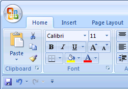
Click
Show Below the Ribbon.
The
Quick Access Toolbar moves beneath the ribbon, as shown below. If
you want to move the Quick Access Toolbar above the ribbon, click
the Customize Quick Access Toolbar list arrow, and then click
Show Above the Ribbon.
|
How To Use the Mini-Toolbar
SUMMARY
Select
the text/object you want to change.
Move
the mouse pointer over the semi-transparent mini-toolbar.
Click
the command or option you want.
|
|
Select some text in a
cell.
A
semi-transparent mini-toolbar appears, as shown below.
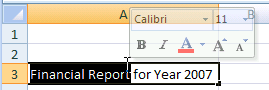
Move
the mouse pointer over the semi-transparent mini-toolbar.
The
semi-transparent mini-toolbar becomes opaque and ready to use, as
shown below.
Click
the command you want.
Excel
applies the quick formatting to the selected text.
|
How To Access The Shortcut Menu Using The Mouse
SUMMARY
Move
the mouse pointer over the cell, text, object or area.
Right-click
the mouse button.
Click
the command you want from the shortcut menu.
|
|
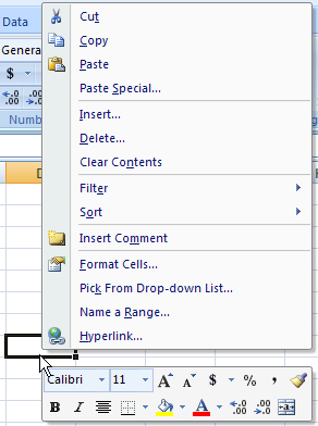
Move your mouse pointer
over any cell in the worksheet.
Before
you click the right mouse button to display the Shortcut menu,
make sure you position the mouse pointer correctly. The location
of the mouse pointer is very important because the Shortcut menu
is context-sensitive. This means that you will display a
different Shortcut menu if you make a right mouse click at a
different location.
Right-click
the mouse. (Click the right mouse button)
A
Shortcut menu appears, as shown below.
Move
your mouse pointer over the Sheet1
tab. Right-click the mouse button.
The
following Shortcut menu appears.
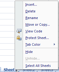
Click
the command you want from the shortcut menu.
Press
<Esc> if you want to cancel the command you clicked.
|
How To Customize The Status Bar
SUMMARY
Right-click
the status bar.
Select
the information you want to add or remove from the status bar.
|
TIPS
The
status bar also let you check the on/off status of Signatures,
Information Management Policy, Permissions, Caps Lock, Num
Lock, Scroll Lock and Fixed Decimal.
|
|
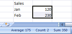
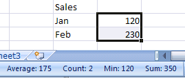
Select the cells
containing the data you want to calculate.
The
average, the number of items selected and the total of the sales
are displayed in the status bar.
Right-click
the status bar.
The
Customize Status Bar menu opens, as shown below.
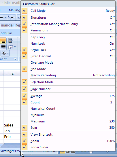
Click
the Minimum
option.
The
minimum of the sales appears in the status bar.
|
How To Change The Views
SUMMARY
Click
the View tab.
In
the Workbook Views
group, click the view you want.
|
TIPS
|
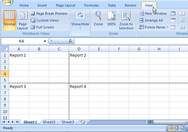
Click the View
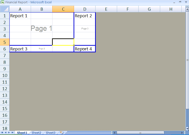
tab.
The
default view is the normal view. Note: We have inserted a page
break, as shown below.
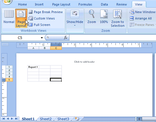
In
the Workbook
Views group, click Page
Layout.
Besides
changing the layout and format of data the way that you can in
Normal view, you can also use the rulers to measure the width and
height of the data, change the page orientation, add/edit page
headers and footers, set margins for printing, and show/hide the
row and column headers. It is useful to get the data ready for
printing.
|
|
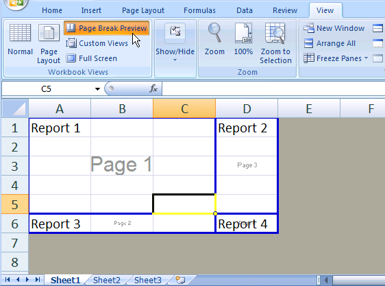
In the Workbook
Views group, click Page
Break Preview.
Page
breaks can be adjusted easily in the Page Break Preview view.
In
the Workbook
Views group, click Full
Screen.
Press
<Esc> to go back to the previous view.
|
How To Show And Hide Workbook Elements
SUMMARY
Click
the View tab.
In
the Show/Hide group, click to select the workbook elements you
want to show or hide.
|
TIPS
|
C lick
the View
tab.
In
the Show/Hide group of the Ribbon, you can see the workbook
elements check boxes, as shown below.
lick
the View
tab.
In
the Show/Hide group of the Ribbon, you can see the workbook
elements check boxes, as shown below.
In
the Show/Hide
group, click to select the elements you want to show or
hide.
Note:
The Ruler is only available in Page Layout view.
|
How To Use The Zoom
SUMMARY
Click
the View tab.
In
the Zoom group,
click the Zoom
button.
Click
the zoom option you want.
Click
the OK button.
|
TIPS
|
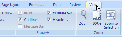
Click the View
tab.
The
Zoom group appears in the Ribbon.
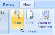
In
the Zoom
group, click the Zoom
button.
The
Zoom dialog box appears.
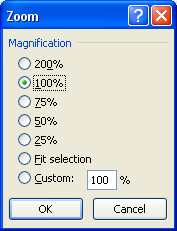
Click
the magnification you want. Then, click the OK
button.
The
worksheet zooms to the magnification you set.
|