Formatting Cells Using The Format Cells Dialog Box

Tab

Description

Number

Specify the format style of the context in a cell.

Alignment

Specify text alignment, text control and text orientation.

Font

Specify font, font style, font size, font color, font effect and underlining.

Border

Specify border color and line style.

Fill

Specify the cell pattern and color.

Protection

Protect the cell by locking it to avoid changes and hiding the formula from the users.

How To Double Underline Using The Menu Option

SUMMARY

1. Select the range A3:A5. You will format the text to have double underlining.

2. Click the Home tab. In the Font group, click the Font dialog box launcher. The Format Cells dialog box appears.

3. Click the Underline drop-down arrow, and click Double from the list. The text in the cells will be double underlined. If you don’t see the underline option, click the Font tab in the dialog box.

4. Click the OK button. The cells format changes as shown below.

How To Align Cell Data Vertically

SUMMARY

1. Select the range B2:C2. You will align the months to the middle of the cell.

2. Click the Home tab. In the Alignment group, click the Alignment dialog box launcher. The Format Cells dialog box appears.

3. Click the Vertical drop-down arrow, and click Center. You can also try other options, if you want.

4. Click the OK button. The months align to the middle of the cells vertically.

How To Change Text Orientation

SUMMARY

TIPS

1. Select the range B2:C2. You will change the text orientation.

2. Click the Home tab. In the Alignment group, click the Alignment dialog box launcher. The Format Cells dialog box appears.

3. In the Degrees box, type 45. You can also click and drag the red diamond shape to change the degrees.

4. Click the OK button. The month’s text orientation changes to 45 degrees anti-clock wise.

5. Change the text orientation again to 90 degrees anti-clock wise. The text orientation of the months changes to the following.

How To Wrap Text In A Cell

SUMMARY

TIPS

1. In the cell A9, type Unit Price in US currency. Then click the confirm button on the formula bar. If you click the confirm button, the active cell remains in cell A9.

2. Click the Home tab. In the Alignment group, click the Alignment dialog box launcher. The Format Cells dialog box appears.

3. Under Text control, click to check the Wrap text check box. The Shrink to fit option is disabled if the Wrap text option is checked.

   Text control options	Description
   Wrap text	Wraps text into multiple lines, depending on the column width and the length of the cell contents in a cell.
   Shrink to fit	Adjusts the font size so that all data in a selected cell fits within the column.
   Merge cells	Combines two or more selected cells into a single cell.

4. Click the OK button. The text wraps within the cell A9.

How To Format Numbers As Currency

SUMMARY

TIPS

1. Select the range C3:C6. You will format the numbers to currency.

2. Click the Home tab. In the Number group, click the Number dialog box launcher. The Format Cells dialog box appears.

3. In the Category box, click Currency from the list. The detailed options for the category appear on the right. Change the options if necessary.

4. Click the OK button. The numbers change to currency. Note: The column is too small to display the contents. You need to enlarge the column width to show the contents. Refer to the Tips on the left for more details.

How To Format Dates

SUMMARY

1. In the cell B10, type Report Date and in the cell C10, type 9/20/07. The cell changes to a date format automatically.

2. Click the Home tab. In the Number group, click the Number dialog box launcher. The Format Cells dialog box appears.

3. In the Category box, click Date. In the Type box, click the 14-Mar-01 format. A preview of the data appears in the Sample area.

4. Click the OK button. The date format changes, as shown below. .

How To Change The Background Color Of A Cell

SUMMARY

1. Select the range A6:C6. You will change the background color of the cells to yellow.

2. Click the Home tab. In the Cells group, click Format >> Format Cells. The Format Cells dialog box appears.

3. Click the Fill tab. Under Background Color, click Yellow from the color palette. You may choose a pattern color and a pattern style if you want.

4. Click the OK button. The background of the cells changes to yellow.

How To Add An Outline Border

SUMMARY

TIPS

1. Select the range A2:D6. You will draw an outline around the selected range.

2. Click the Home tab. In the Cells group, click Format >> Format Cells. The Format Cells dialog box appears.

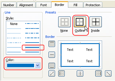
3. Click the Borders tab. Under Line, in the Style box, select a thick line style. Click the Color drop-down arrow and select blue. Under Presets, click the Outline button. The selected options appear as shown below.

4. Click the OK button. An outline is added to the selected range.

How To Add A Double Line Border

SUMMARY

1. Select the range A3:D3. You will draw a double border at the top of the selection.

2. Click the Home tab. In the Cells group, click Format >> Format Cells. The Format Cells dialog box appears.

3. Click the Borders tab. Under Line, in the Style box, click the Double Line style. Under Border, click the Top Border button. The border settings are shown below.

4. Click the OK button. A double borderline appears at the top of the selection.

How To Draw A Border Using The Mouse

SUMMARY

TIPS

1. Click the Home tab. In the Font group, click the Borders drop-down arrow. A list of draw borders options appears.

2. Move you pointer over the Line Color. Then, click Line Color >> Red color. You can also set the line style by moving your pointer to the Line Style. Then, click to select the line style you want from the submenu. The pointer will change to a pen automatically. You can then start to draw the borders.

3. Draw the borders. Press <Esc> when you want to stop drawing. If you need to erase any unwanted borders, click Erase Border from the list and then erase the borders you want.

How To Format A Table Quickly

SUMMARY

1. Select the table range A2:D6. You will apply a predefined table style to the selected table.

2. Click the Home tab. In the Style group, click the Format as Table button. A list of table style appears.

3. Click the Table Style Light 9. The Format As Table dialog box appears.

4. Click the OK button. The style is applied to the selected table.