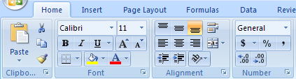
Formatting Cells Using The Ribbons
Excel
allows you to control the appearance of the cells. This includes the
data format, font, alignment, border, and fill of the cells.

How To Change The Font
SUMMARY
Select
the cell, in which you want to change the font.
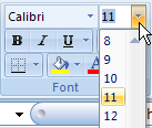
Click
the Home tab. In
the Font group,
click the Font
drop-down arrow.
Click
the font you want from the list.
|
|
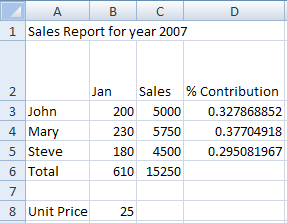
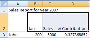
Select the range B2:D2,
in which you want to change the font.
The
cells are highlighted.
Click
the Home
tab. In the Font
group, click the Font
drop-down arrow.
A
list of the font types appears.
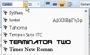
Click
Times
New Roman from the list.
Note:
scroll down the list to find the font you want if necessary. The
font in the range B2:D2 has changed.
|
How To Change The Font Size
SUMMARY
Select
the cells you want to change.
Click
the Home tab. In
the Font group
To
change font size: Click the Font
Size drop-down arrow.
To
make text bold:
Click
 or press <Ctrl>+<B>
To
Italicize text:
Click
or press <Ctrl>+<B>
To
Italicize text:
Click
 or press <Ctrl>+<I>
To
underline text:
Click
or press <Ctrl>+<I>
To
underline text:
Click
 or press <Ctrl>+<U>
To
change the font color:
Click the
or press <Ctrl>+<U>
To
change the font color:
Click the
 drop-down
arrow and click the color you want.
drop-down
arrow and click the color you want.
|
|
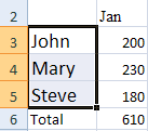
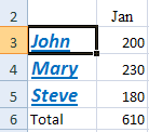
Select the range
A3:A5.
You
want to format the sales persons’ names.
Click
the Home
tab. In the Font
group, click the Font
Size drop-down arrow.
A
list of the font sizes appears.
Click
12
from the list.
The
font size in the range A3:A5 has changed.
|
How To Make Text Bold
|
Click the
Bold
button.
|
How To Italicize Text
|
Click the
Italic
button.
|
How To Underline Text
|
Click the
Underline
button.
|
How To Change The Font Color
SUMMARY
Select
the cells you want to change.
Click
the Home tab. In
the Font group.
Click
the Font Color
drop-down
arrow and click the color you want.
|
|
Select the range
A3:A5.
You
want to format the sales persons’ names.
Click
the Home
tab. In the Font
group, click the Font
Color drop-down arrow.
The
Font Color Palette appears.
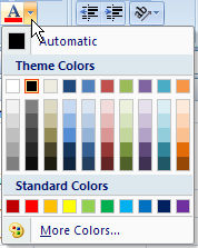
Click
the Blue
color.
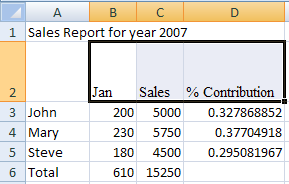
The
font is formatted as shown below.
|
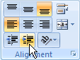
How To Align Data In A Cell
SUMMARY
Select
the range you want to align.
Click
the Home tab. In
the Alignment
group, click the following button.
To
align center,

To
align left

To
align right

|
TIPS
You
can also
Justify
Align
the data in the cell.
Select the range.
Click the
 dialog
box launcher
at the Alignment
group. Click the Alignment
tab. Under Text
alignment,
in the Horizontal
box, click Justify.
dialog
box launcher
at the Alignment
group. Click the Alignment
tab. Under Text
alignment,
in the Horizontal
box, click Justify.
|
|
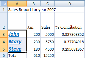
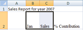
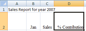
Select the range B2:C2.
You
will align the content in the range to the center.
Click
the Home
tab. In the Alignment
group, click the Center
button.
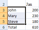
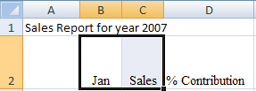
 The
cell content is aligned to the center horizontally.
The
cell content is aligned to the center horizontally.
-
Alignment
Button
|
Description
|
Align
Center
|
Aligns
cell content to the center.
|
Align
Left
|
Aligns
cell content to the left.
|
Align
Right
|
Aligns
cell content to the right.
|
|
How To Indent Data In A Cell
SUMMARY
To
Increase indent, click

To
decrease indent, click

|
|
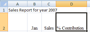
Select the cell
D2.
You
want to increase the indentation of the content in the cell.
C
lick
the Home
tab. In the Alignment
group, click the
 Increase
Indent button.
The
indentation in the cell has increased. Click the Increase Indent
button a few times to increase the indentation further.
To
decrease the indentation, click the
Increase
Indent button.
The
indentation in the cell has increased. Click the Increase Indent
button a few times to increase the indentation further.
To
decrease the indentation, click the
 decrease
indent button.
decrease
indent button.
|
How To Merge Cells
SUMMARY
Select
the cells you want to merge.
Click
the Home tab. In
the Alignment
group, click the Merge And Center
button.
|
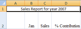
|
Select the range
A1:D1.
You
will align the title of the table to the center of the entire
table width.
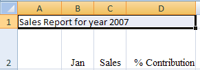
C
lick
the Home
tab. In the Alignment
group, click the
 Merge
And Center button.
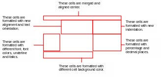
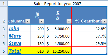
The
selected cells are merged and the title of the table is aligned
to the center of the merged cells.
Merge
And Center button.
The
selected cells are merged and the title of the table is aligned
to the center of the merged cells.
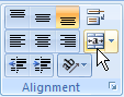
 To
see more merge options, click the merge & center drop-down
arrow, as shown below.
To
see more merge options, click the merge & center drop-down
arrow, as shown below.
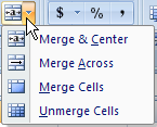
-
Merge
Options
|
Description
|
Merge
& Center
|
Merge
the selected cells and align the content to the center
horizontally.
|
Merge
Across
|
Merge
the selected cells in the same row.
|
Merge
Cells
|
Merge
all the selected cells.
|
Unmerge
Cells
|
Unmerge
the cells.
|
|
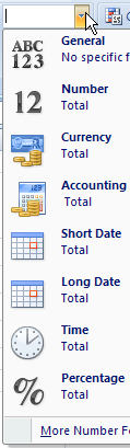
How To Change Numbers To Percentages
SUMMARY
Select
the cells containing the numbers you want to change to
percentages.
Click
the Home tab. In
the Number group,
click the
 Percentage
button.
Percentage
button.
|
|
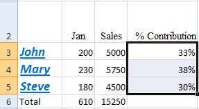
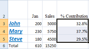
Select the range
D3:D5.
The
selected numbers will be changed to the percentage format.
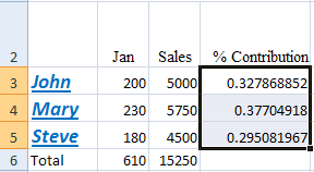
C
lick
the Home
tab. In the Number
group, click the
Percentage
button.
 The
numbers are changed to percentages with
no decimal
places.
The
numbers are changed to percentages with
no decimal
places.
|
How To Increase / Decrease Decimal Places
SUMMARY
To increase decimal
places
Select
the cells containing the numbers you want to change.
Click
the Home tab. In
the Number group,
click the
 Increase Decimal
button.
Increase Decimal
button.
To decrease decimal
places
Select
the cells, containing the numbers you want to change.
Click
the Home tab. In
the Number group,
click the
 Decrease Decimal
button.
Decrease Decimal
button.
|
TIPS
|
Select the range
D3:D5.
You
will increase and decrease the decimal places.
C
lick
the
Increase
Decimal button twice.
 The
numbers now have two decimal places.
The
numbers now have two decimal places.

Click
the
Decrease
Decimal button.
The
numbers change to one decimal place.
|
How To Copy A Format Using Format Painter
SUMMARY
Click
the cell, for which you want to copy the format.
Click
the Home tab. In
the Clipboard
group, click the
 format painter
button.
format painter
button.
Select
the cells, to which you want to paste the format.
|
TIPS
You
can only paste the copied format once if you click the Format
Painter
button once.
If
you want to paste the format you copy to multiple non-adjacent
cells or ranges, double-click
the Format
Painter
when you copy the format.
After you finish, press <Esc>
to disable the format painter.
|
|
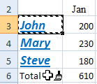
Select the cell
A3.
You
will copy the format of the cell A3.
Click
the Home
tab. In the Clipboard
group, click the
Format
Painter button.
The
format of the cell A3 is copied and your mouse pointer changes to
a format painter.

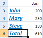
C
lick
the cell
A6 to paste the format.
The
format of cell A3 is pasted to cell A6, as shown below. You can
also click and drag to paste the format onto a range of cells.
|


 .
.