Adjusting Column Width / Row Height
The
column width and the row height of a worksheet may be modified to
improve the worksheet’s appearance. The row height is adjusted
automatically when you change the size of the cell content. You can
also adjust the appearance manually with the mouse or the Ribbon.
You
can set a column width of 0 (zero) to 255, which indicates the number
of characters that can be displayed in a cell (in the condition that
the cell is formatted with the default standard font). The default
column width is 8.43 characters.
Note:
If a column has a width of 0 (zero), the column is hidden.
You
can set a row height of 0 (zero) to 409, which represents the height
measurement in points. The default row height is 12.75 points
(approximately 1/6 inch or 0.4 cm).
Note:
If a row has a height of 0 (zero), the row is hidden.

How To Adjust The Column Width Using The Mouse
SUMMARY
Position
your mouse pointer at the boundary on the right of the column
heading of which you want to adjust the width.
Click
and drag to the width you want.
|
TIPS
To
AutoFit the width of a column
- double-click at the right boundary of the column
heading
or
- Select the column, click the Home
tab, in the Cells
group, click the Format
button. Then click AutoFit
Column Width.
To
adjust the width of multiple columns,
select the columns you want, and then drag any column-heading
boundary within the selection.
|
|
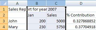
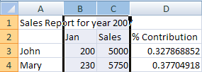
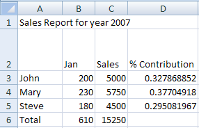
Before you begin, create
the following worksheet.
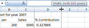
Position your mouse
pointer at the boundary on the right of the Column
D heading.
This
is to adjust the column D width. The pointer changes to a
double-headed arrow, as shown below.
Click
and drag to the width you want.
The
column width information is shown when you drag the boundary.
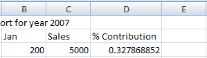
Release
the mouse button.
The
column width is adjusted as shown below.
|
How To Adjust The Column Width Using The Menu
SUMMARY
Select
the columns, for which you want to adjust the width.
Click
the Home tab. In
the Cells group,
click the Format
button.
Click
Column Width. In
the Column width
box, type the new width you want.
Click
the OK button.
|
|
Select Column
B and Column
C.
Click
at the column heading B and drag to column C to select the
columns.
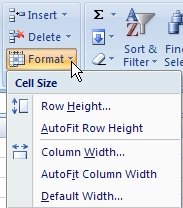
Click
the Home
tab. In the Cells
group, click the Format
button.
A
list of options appears, as shown below.
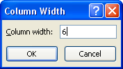
Click
Column
Width. In the Column
width box, type 6.
A
Column Width dialog box appears, as shown below.
Click
the OK
button.
The
width of the selected columns is adjusted.
|
How To Adjust The Row Height Using The Mouse
SUMMARY
Position
your mouse pointer at the boundary below the row heading of
which you want to adjust the height.
Click
and drag to the height you want.
|
TIPS
To
AutoFit the height of a row
- double-click at the boundary below the row
heading
or
- select the row, click the Home
tab, in the Cells
group, click the Format
button. Then click AutoFit
Row Height.
To
adjust the height of multiple rows,
select the rows you want, and then drag any row-heading
boundary within the selection.
|
|
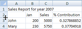
Position your mouse
pointer at the boundary below the Row
2 heading.
This
is to adjust the height of row 2. The pointer changes to a
double-headed arrow, as shown below.
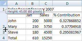
C lick
and drag to the height you want.
The
new row height appears near the mouse pointer when you drag the
boundary.
lick
and drag to the height you want.
The
new row height appears near the mouse pointer when you drag the
boundary.
|
How To Adjust The Row Height Using The Menu
SUMMARY
Select
the row.
Click
the Home tab. In
the Cells group,
click the Format
button.
Click
Row Height. In the
Row height box,
type the new height you want.
Click
the OK button.
|
|
Select the row
2.
Click
the row 2 heading.
From
Click the Home
tab. In the Cells
group, click the Format
button.
A
list of options appears, as shown below.
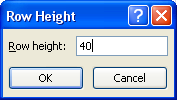
Click
Row
Height. In the Row
height box, type 40.
A
Row Height dialog box appears, as shown below.
Click
the OK
button.
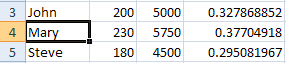
The
row height is now adjusted.

|
How To Hide / Unhide Rows / Columns
SUMMARY
Select
a cell or cells that you want to hide/unhide.
Click
the Home tab. In
the Cells group,
click the Format
button.
To Hide Rows,
Click
Hide & Unhide >> Hide
Rows.
To Hide Columns
Click
Hide & Unhide >> Hide
Columns.
To Unhide Rows
Click
Hide & Unhide >> Unhide
Rows.
To Unhide Columns
Click
Hide & Unhide >> Unhide
Columns.
|
|
Click cell
A4.
You
will hide Mary's data.
Click
the Home
tab. In the Cells
group, click the Format
button.
A
list of options appears, as shown below.
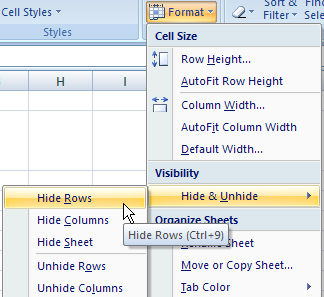
Click
Hide
& Unhide >> Hide Rows.
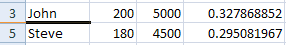
The
entire row 4 disappears.
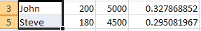
Click
and drag to select A3:A5.
You
need to select the cells on either side of the hidden row or
column.
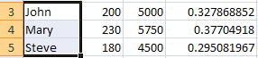
In
the Cells
group, click the Format
button. Click Hide
& Unhide >> Unhide Rows.
Row
4 reappears, as shown below.
|
How To Freeze A Column / A Row
SUMMARY
Click
the cell to the right of the columns you want to freeze,
or/and below the rows you want to freeze.
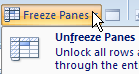
Click
the Home tab. In
the Cells group,
click the Freeze Panes
button.
Click
Freeze Panes.
|
TIPS
Note:
You will only see the Unfreeze Panes command after freezing
panes.
|
|
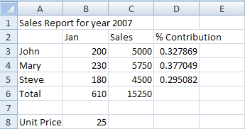
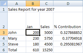
Click cell
B3.
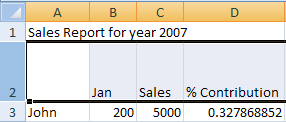
You
will freeze column A and row 2, so that when you scroll down, the
sales person names and the column titles remain on your screen.
Click
the Home
tab. In the Cells
group, click the Freeze
Panes button.
A
list of options appears, as shown below.
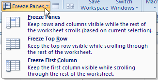
Click
Freeze
Panes.
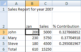
Black
lines appear on the left and above the active cell.
-
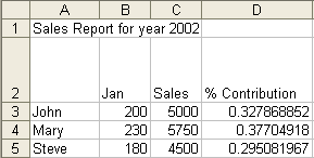
When
you scroll down your screen, the column titles remain on your
screen.
|
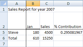
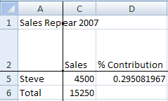
When
you scroll to the right of your screen, the sales person names
remain on your screen.
|
|
How To Split A Worksheet Into Panes
SUMMARY
Click
the cell where you want to split the worksheet.
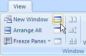
Click
the View tab. In
the Window group,
click the Split
button.
|
TIPS
|
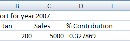
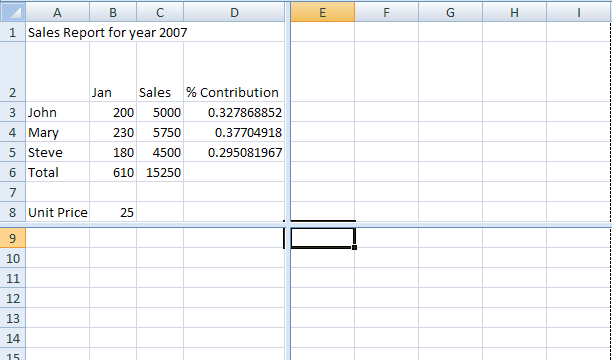
Click cell
E9.
The
worksheet will split at the position of the active cell E9.
Click
the View
tab. In the Window
group, click the Split
button.
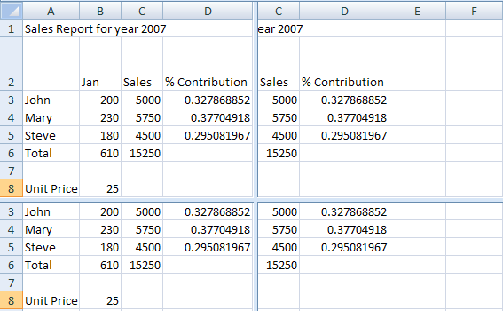
 The
worksheet window splits into 4 panes, as shown below.
The
worksheet window splits into 4 panes, as shown below.
 Use
the vertical and horizontal scroll bars to show the data in the
empty panes. You can fill the other panes with the data from
different parts of the worksheet.
Use
the vertical and horizontal scroll bars to show the data in the
empty panes. You can fill the other panes with the data from
different parts of the worksheet.
|