Identifying Dimensions of a Construct

The term dimension can also be used to describe groups of variables that all measure basically the same thing but in slightly different ways. For example, we might decide that there are three dimensions6 of the construct media use:

Dimension 1. Amount of exposure to each of the media

Dimension 2. Types of content the audience reads/views/listens to

Dimension 3. Functions that the media fulfill

But each dimension could also be broken down into one or more variables. For example:

Dimension 1. Amount of exposure to each of the media

Variable la. Days per week people use each of the media Variable lb. Minutes per day people use each of the media Variable lc. Number of media people read/view/listen to per day

Dimension 2. Types of content the audience reads/views/listens to Variable 2a. Attention to specific types of content Variable 2b. Frequency of exposure to specific types of content

Dimension 3. Functions that the media fulfill

Variable 3a. Extent to which a person reads/views/listens to each of the media to get information about what's happening in the world

Variable 3b. How successful each of the media is in fulfilling this function

In this example, we might want to reduce the number of variables— seven in all—by creating an additive index that would represent the dimensions by combining the individual variables that are a part of each dimension. This would leave us with three variables (the indexes that represent the three dimensions) instead of seven (the number of individual variables in all dimensions). We'll talk more about indexes later in this chapter.

• DEFINING CONCEPTS

Once we have decided which concepts to use, we must define them, both theoretically and operationally. These two ways of looking at con­cepts provide information about both meaning and measurement.

Theoretical Definitions

The theoretical definition (sometimes called the conceptual definition) conveys the meaning we attach to the concept and generally suggests indicators of it. We could think of the theoretical definition as the "dic­tionary" definition and of the indicators as "hints" about how the con­cept might be measured. Each concept can have a variety of meanings, so it is up to the researchers to specify which meaning they intend.

For example, the construct we used above, media use, can be theo­retically defined as "an individual's readership, viewership, or listen- ership to the content of television, newspapers, magazines, radio, and the Internet, such as [indicators] exposure, content used, or functions fulfilled." Note that the end of the definition suggests some indicators of the construct, so our job isn't done: These indicators have identified three potential dimensions of media use, and we must also theoretically define each:

• Frequency of audience exposure to media—the extent to which an individual reads/views/listens to television, newspapers, magazines, radio, or the Internet during a specified time frame, such as [indicators] days per week, minutes per day, or the number of each that is used each day

• Types of content the audience reads/views/listens to—the extent to which people consume certain specified types of content (e.g., sports, news, and public affairs), such as [indicators] the amount of atten­tion that the person pays to the specified content or the amount of such specific content that they read/view/listen to within a specified time frame

• Functions that the media fulfill—the extent to which people identify television, newspapers, magazines, and radio with certain gratifica­tions (e.g., entertainment, surveillance), such as [indicators] reasons why each medium is used or the extent to which each medium gives people what they want

Multiple Indicators of a Concept

The use of multiple indicators within the theoretical definition for each concept helps us understand that each concept has a variety of meanings. In the example above, although we have suggested several indicators for each concept, these indicators can never measure all of the meaning implied by the theoretical definition. Hage (1972) uses the term meaning space to indicate the universe of indicators that a concept can take. Usually we mean more by a concept than we can measure at once. As Figure 2.1 shows, using even three indicators of a concept cannot tap all of the meaning of the concept.

Although using multiple indicators does increase the amount of the concept's meaning that is being measured, some of the indicators may be more valid than others.

Theoretical Validity of Indicators

Validity is the extent to which the indicators measure the concept we think we are measuring. We often find that we cannot use all of the indicators available in our studies and must therefore identify the ones that are most valid—that best measure the concept. Sometimes it's dif­ficult to decide which indicators are most valid, however. How broad or specific should the concept be? How do we know which indicators are the best measures of the concept?

For example, let's say we are interested in testing the hypothesis "Watching television makes children perform less well in school." There are two major concepts: television watching and academic perfor­mance. We could define television watching as the extent to which a child is exposed to the content of television, such as

• Hours per day the child watches television

• Number of programs watched per day

• Preference for television viewing over reading or other activities

We could define academic performance as the extent to which the child does well in school or school-related work, such as

• Grades on child's most recent report card

• Teacher's other evaluation of child's academic performance

• Standardized test scores

Amount of time per day child spends doing homeworkFigure 2.1 Meaning space of a concept. A concept is never completely measured, no matter how many variables are used. In this example, the first three variables are shown to measure part of the concept, and creating a new variable (minutes/week = days/ week times minutes/day) adds a bit more to measured meaning. However, the white block indicates that some meaning of the concept media use remains unmeasured. Theoretically, this is always the case.

Legend

Щ Days/week used the media JJj Minutes/day used the media | | Number of media used КлхЯ Days/week times minutes/day

Part of concept media use unmeasured by the above variables

SOURCE: Adapted from Hage (1972, p. 64).

The decision about which indicators to use will have a profound effect on the result of the study. For example, we know that the California Achievement Program's 1980 study (Comstock & Paik, 1991) used the actual hours per day spent viewing television as a measure of television watching and percentage of time doing homework as a measure of predicted academic performance. Using these two indica­tors does show that these concepts are positively related (i.e., the more television a child watches, the lower the child's academic perfor­mance). But other indicators studies using these indicators sometimes have resulted in the finding of no relationship. Faced with such contradictory findings, we would need to evaluate the validity of our indicators and perhaps do a third study with indicators we considered more valid.

Instead of the general concept television watching, we might want to specify our concept as exposure to television entertainment programs. Instead of the general concept academic performance, we might want to specify the amount of time spent doing homework. Our hypothesis would become "The more entertainment television programs a child watches, the less time the child will spend doing homework." Then we could investigate whether one or both of these variables were related to the child's academic performance.

Operational Definitions

Although the indicators in the theoretical definition hint at ways in which the concept may be measured, the full measurement scheme is specified in the operational definition—complete and explicit information about how the concept will be measured. This term can be confusing, because the word definition doesn't bring measurement to mind.

Whereas theoretical definitions all look much the same—like a dictionary definition—the form that operational definitions take will depend on the research method being used. Processes and procedures of variable measurement and data collection sometimes vary dramatically in various research methods because they are designed to answer differ­ent types of questions and test different types of hypotheses. We will look at examples of operational definitions for three research methods.

Operational Definitions in Survey Research

In a survey, the operational definition will probably be the text of a question and its possible responses. To measure local television news exposure, we might ask:

• How many days a week do you watch local television news? DAYS

• On an average day, how much time do you spend watching local television news? CODE IN MINUTES

Then we could multiply days by time per day to get how many minutes per week local television news is viewed.

To measure newspaper credibility, we might try to tap several aspects of the construct—fairness, balance, and objectivity:

• The Gazette is fair in its coverage of my community.

4. Strongly agree

4. Agree

3. Neutral

2. Disagree

1. Strongly disagree

• The Gazette gives balanced coverage to different groups in my

community.

4. Strongly agree

3. Agree

3. Neutral

2. Disagree

1. Strongly disagree

• The Gazette's coverage of my community is objective.

3. Strongly agree

4. Agree

3. Neutral

2. Disagree

1. Strongly disagree

Each dimension of media credibility is measured using the same scale (see Babbie, 1998, pp. 141-145), and each can be considered an operational definition. It is also possible to combine the dimensions as measuring the construct credibility, as we will see at the end of this chapter.

Operational Definitions in Experiments

Variables in experiments are either manipulated or measured, and the type of operational definition will differ for each.

Manipulated variables in experiments are independent variables. The researcher creates an experimental treatment group for each value of the independent variable and then (in a randomized experiment) randomly assigns subjects to treatment groups. The researcher then manipulates or determines which treatment group gets each value of the independent variable. For example, we could test the hypothesis "Children who see a violent television show act more aggressively than those who see a nonviolent show." The manipulated variable would be amount of violence, which the hypothesis implies would have two values—violent and nonviolent. Thus, we would need two treatment groups and two television shows. If we had access to a group of children, we could flip a coin to determine which treatment group each child was in. This is a simple operational definition for the manipu­lated independent variable. A better operational definition would describe more about the television shows and how the level of violence was determined. The point is to completely describe how the manipu­lated variable is being measured.

Measured variables' operational definitions in experiments can take several forms. Sometimes a questionnaire is used to gather demo­graphic information (e.g., sex, age, ethnicity) or to measure attitudes or knowledge. These may be independent or dependent variables, depending on the hypotheses being tested in the experiment. (Obviously, a person's sex or age is unlikely to be changed in an exper­iment, so these would be used as independent or control variables.) Other methods of measurement include observation, apparatuses that measure the time it takes a subject to hit a button, blood pressure, brain waves, and many more. In the example hypothesis above, we could measure the dependent variable, aggressive behavior, by observing children on a playground after (and perhaps before) they saw the films. We could create a list of behaviors considered aggressive, assign a coder to watch each child, and count the number of times each child exhibited each behavior. We could finish the operational definition by summing the total number of aggressive behaviors for each child, or we could further weight each behavior by how much aggression it rep­resented. For example, here's how these types of aggressive behaviors might be weighted:

10. Making another child fall

9. Kicking

8. Hitting

3. Biting

4. Shoving

4. Tripping

2. Pulling hair

1. Yelling

A complete operational definition measuring aggression would have to indicate where the list and numerical measurement of aggres­sive behaviors came from and to demonstrate both that it was exhaus­tive and that the values were mutually exclusive. The operational definition would also have to specify and justify the weighting system and show how it would be applied. Generally, the number of times each behavior is exhibited would be multiplied by its weight, then the scores for each subject summed:

3 hits x weight 8 = 24 points

1. shove x weight 4 = 4 points

10 yells x weight 1 = 10 points

The total represents an aggression score of 38 points for this child, which could be compared to other children's scores. A score of 0 would indicate that no aggressive acts were observed.

Operational Definitions in Content Analysis

In content analysis studies, variables can be categorized as either content or noncontent. Content variables are those messages being analyzed, such as newspaper articles, television shows, films, or per­sonal correspondence. These are often dependent variables. Noncontent variables are sometimes used as predictors (independent variables) of content, other times as outcomes (dependent variables). For example, Shoemaker (1984) tested the hypothesis "The more deviant journalists rate political groups, the less legitimately the groups will be covered by newspapers." Deviance (the noncontent, independent variable) was measured by surveying editors at the 100 largest newspapers about their attitudes toward 11 political groups. Legitimacy was measured with a content analysis of more than 500 articles from several newspapers. In another example, Shoemaker et al. (1989) tested an agenda-setting hypothesis: "The more the media emphasize drugs, the more people think drugs are the most important problem facing the country." They used Gallup Poll public opinion data (the percentage of people who named "drugs" as the most important problem facing the country) as the noncontent, dependent variable. The independent variable was measured by counting the number of stories about drugs in three newspapers, three television networks, and three newsmagazines.

Content variables generally have very complicated operational definitions because they have to describe the entire process of selecting the content (e.g., newspapers) to be studied: selecting the unit of analysis, the recording unit, and the context unit (Holsti, 1969) and describing the rules to be used in coding. This will almost certainly require several pages of description.

Noncontent variables may be measured by gathering data using some other research method, such as survey research, or data may be used from various archives, such as the U.S. Bureau of the Census, the Statistical Archives of the United States, or more specialized sources such as Gallup Poll data or film ratings from the Motion Picture Association of America. An increasing amount of archival data is avail­able on the Internet or from various online subscription services such as Nexis. Noncontent operational definitions must include complete infor­mation about the other data-gathering operation or the archival data source. The goal is to provide enough information to allow someone else to replicate the study and also to ensure that the reader can evalu­ate the reliability and validity of the source's data-gathering methods.

Building Scales and Indexes

So far we have discussed specifying operational definitions for one variable at a time, but we have also made a case for the use of multiple indicators of a concept. In the content analysis example above by Shoemaker (1984), the concept deviance was initially theoretically defined with four indicators, and the concept legitimacy with 17 indica­tors. Though having multiple indicators of each concept is desirable, it would be impractical to use each indicator as a separate variable in the data analysis—the result would be 68 tests of the same hypothesis, using all possible combinations of all variables. Although it is cer­tainly possible to do this, it seems a bit absurd. Also, interpretation of the results would be difficult if, for example, 8 of the 68 tests did not support the overall hypothesis: Could the authors conclude that the hypothesis was supported?

An alternative is to collect the data for all 21 variables but in data analysis to combine them into theoretically related concepts. Such composites are called scales or indexes, the most common of which is the result of summing the responses to two or more variables. A good scale or index will be unidimensional, have a reasonable amount of variance, and have face validity (Babbie, 1998). The terms scale and index are often used interchangeably, and these labels are even applied to operational definitions of single variables. For example, the term Likert scale (strongly agree to strongly disagree) is often applied both to the responses to a single variable and to composite variables in which several vari­ables using this operational definition are added together. Conversely, Cronbach's alpha is a commonly used measurement of the reliability of an additive composite construct, which in the procedure is referred to as a scale. Nonetheless, in this book we will use the term index when we are referring to composite measures of concepts. We use the term scale when we are referring to the measurement (operational definition) of a single variable.

In the earlier example, Shoemaker (1984) created five indexes out of the 21 variables she used in data collection. The deviance index was created by summing journalists' responses to four questions measuring their attitudes toward 11 political groups. The statistical procedure factor analysis was used to look for the existence of multiple dimen­sions among the 17 measures of legitimacy. Four dimensions were revealed and were labeled evaluation, legality, viability, and stability. Four indexes were created by summing responses to the variables within each dimension.

The factor analysis process helps us look at whether the 21 variables are unidimensional or multidimensional: that is, whether they represent one concept in common or whether they represent several concepts that act as dimensions of an overall construct. Because one characteristic of a good index is unidimensionality, this is important information. The four dimensions that Shoemaker found suggested that the construct legitimacy is multidimensional. Therefore, four summative and uni­dimensional legitimacy indexes and the summative deviance index were created, resulting in 5 variables for data analysis instead of 21. Before summative indexes can be used, however, we must ascertain whether each index is itself unidimensional. Cronbach's alpha assesses the probability that each item in the index measures the same underly­ing concept. Alpha ranges from .00 to 1.00, and the higher the coefficient, the more reliable the index is. An index that is not unidimensional—that measures more than one concept—will have a low alpha.7

Indexes also need adequate variance and face validity. To be valid on the "face of it" means that the index's component variables appear as if they all are measuring the same thing. Variance can be assessed through simple data analysis that shows the distribution of values in the index and how many cases fall in each. If the vast majority of cases are clumped together on a few values, this may indicate that the index will be of limited value in hypothesis testing. An index with limited variance will not relate well to other variables, regardless of its theo­retical validity. One can also look at dispersion statistics, the variance, standard deviation, and range, although these are most valuable when comparing one variable's variance with another.

• NOTES

1. As we will argue later, this is not a good way of measuring the variable education because it breaks a continuous variable into four large categories.

2. Admittedly, using biological sex as an independent variable doesn't give us much explanatory or predictive power. As we will discuss later in this chapter, categorical variables such as gender are often surrogates for continuous variables such as motivation, interest, usefulness, and so on, and these would provide more explanatory and predictive power.

3. In Shoemaker et al.'s (1989) study of public opinion and media coverage about drugs, public opinion was in fact a variable. Studies in which a concept that is assumed to be a variable turns out to be a nonvariable rarely are pub­lished. A lack of variance generally results in null findings—a lack of statistical support for the research hypothesis.

4. As we will discuss in detail in Chapter 3, the hypothetical form "The more..., the more..." implies that the first concept mentioned is the inde­pendent variable. In this case, we could just as easily have said, "The more interested people are in politics, the more they read a daily newspaper."

5. For more information on levels of measurement, see Babbie (1998, pp. 141-145).

6. In this example, each dimension is also obviously a concept; however, the term dimension implies that multiple concepts can be used to represent a construct. These groups of concepts can be referred to as dimensions of the construct.

Although we show the standard Likert scale here, it is important to remember that some people will reply don't know or will refuse to answer the question. These categories are routinely added to the coding scheme (although less often offered to the respondent) as 8 = don't know and 9 = refuse. Also, the assignment of the values (e.g., 1 = strongly disagree instead of strongly agree) is determined theoretically. The "most" of the concept as used in the hypothesis is generally assigned the largest valid value (e.g., 5 = strongly agree if the con­cept is agreement). The codes 8 and 9 are not considered "valid" because they do not represent any amount of agreement. In the case of the Likert scale, they represent types of nonresponse.г

3

Theoretical Statements Relating Two Variables

e

_W

said in the previous chapter that a hypothesis must be made up of at least two variables; a hypothesis expresses the relationship between two or more variables. We also referred to assumptions and propositions. In this chapter, we look at the relations between two vari­ables more closely and distinguish among several types of theoretical statements.

Hage (1972) suggested that the term theoretical statement be used to describe more broadly the relationship between variables, encompass­ing such terms as assumption, hypothesis, postulate, proposition, theorem, and axiom. In this book, we will use three of the more specific terms— assumption, hypothesis, and proposition—with theoretical statement being used generally to describe all three.

A theoretical statement says something about the values of one or more variables, although it is generally thought of as expressing some­thing about the relationship between two or more variables (e.g., "The more television a child sees, the more aggressive the child will act"). Other kinds of theoretical statements describe the values of only one variable (e.g., "There is a consistently high amount of violence on prime-time television").

We find it useful to distinguish among three types of theoretical statements:

Hypothesis—A testable statement about the relationship between two or more concepts (variables):1 for example, "The more politi­cally active people are, the more time they spend reading a daily newspaper." Testable means that social science research methodol­ogy and statistics can be applied to discover the extent of support for the statement.

Assumption—A theoretical statement that is taken for granted, not tested. The assumption may describe the relationship between variables (similar to a hypothesis, above), or it may describe the usual value of one variable in a given situation (as in propositions, below). Some assumptions may be considered untestable or may be beyond the scope of the study: for example, "The more rational the electorate, the more it is motivated to seek political information in the mass media." Others could be tested, but are taken for granted in a given study: for example, "The more politically active people are, the more motivated they are to get information about the election from the mass media." Such assumptions are often used as theoretical linkages for hypotheses: that is, reasons why the hypothesis may be supported.

Propositions are less useful than theoretical statements that address the relationship between two or more variables because they are merely descriptive and provide information about only one variable at a time: for example: "The free flow of information is valuable in a democracy." Propositions often take on a normative tone, in which scholars state how things should be, according to their ideological views.

• IDENTIFYING ASSUMPTIONS

Whether assumptions are propositional or relational, it is crucial for the social scientist to specify as many assumptions underlying the research and theory as possible. Assumptions are necessary (not everything can be tested) and/or convenient (pragmatism requires that not every scholar go back to the ultimate cause, e.g., the big bang). All studies are based on one or more underlying assumptions. These form the logical rationale for the study and can be used to derive the hypotheses. Although the reader does not require, for example, an assumption of evolutionary biology when reading a study of most human behavior, it is helpful for scholars to clarify their own deeply help beliefs and to acknowledge these when directly pertinent to the study. The more scholars can identify the assumptions that underlie their theories and research, the more they and others can understand the implications of the theories. If the reader does not agree with the basic assumptions underlying the research, then the rest of the work is called into ques­tion. Therefore, identifying and communicating assumptions is a form of intellectual honesty. Sometimes assumptions are not or cannot be made explicit by the researcher, and it is up to the reader to identify them.

Unfortunately, identifying and stating assumptions is one of the most difficult parts of theory building because the things we take for granted are part of our individual ideological and normative systems and are therefore transparent to our daily thought processes. Such preconscious ideas have a direct effect on the research conducted. Consider ideas such as:

• Capitalism is the best economic system.

• Men are more capable than women are.

• The unemployed lack the intelligence or motivation to find and hold jobs.

• The United States operates as a democratic political system.

• The more information people can have about political candi­dates the better.

• Mass media content basically mirrors reality.

• Newspapers provide more information about an election than television news programs.

Many people may agree with such statements, but establishing informal agreement is not science. Most people used to agree that the sun orbited the earth, but agreement did not make it true, and it took scientific observation to show the opposite.

Science advances by testing of hypotheses, not by assuming that certain things are true. Assumptions can be challenged on logical or philosophical grounds, but in this case one person's opinion may be as valid as another's. Social science methods and statistics provide a potentially more objective form of evaluating the relative support for a hypothesis. These methods attempt to be independent of a given scholar's personal biases and may be replicated by others. If they are replicated, we have more confidence in the original hypothesis test. Scientists recognize that no one is completely without bias and that too much bias can negatively influence the outcome of studies. Researcher bias is a threat to establishing internal validity: that is, showing that changes in the dependent variable are due to the independent variable and not to other causes.

As we indicated in the previous chapter, Hage (1972) suggested that the use of categorical variables may signal underlying assump­tions that need to be specified. Why compare men's voting or news­paper reading to women's? What distinguishes men from women that makes us think that they will vote or read differently? Could there be assumptions about political interest, intelligence, and ability to under­stand abstract concepts, availability of time and transportation? If we can ask "why" when categorical variables are proposed, we may be able to uncover underlying assumptions, turn them into hypotheses, and actually test the extent to which assumptions are supported.

The lower the proportion of assumptions to hypotheses a theory has, the more it explains about the phenomenon at hand. Tested and supported hypotheses provide information about what the world is like. This is not the same as reaching truth, as Popper (1968, 1972) cautioned, but repeated hypothesis tests with consistent results do give us some reassurance about their validity. Assumptions, however, are mere guesses about the nature -of the world and have no scientific support. What "everybody knows" may in fact be incorrect. Therefore, the fewer assumptions a theory contains relative to the number of hypotheses, the more power the theory has to describe, explain, and predict the world in a way than can be empirically defended.

• FORMS OF HYPOTHESES

Hypotheses that express the relationship between two variables can be written in a wide variety of ways, some more intelligible than others. Basically, hypotheses tell us something either about the difference between the average values of variables (e.g., A is on the average bigger than B) or about the relationship between two variables' values (e.g., as the values of A change, the values of В also change).

A hypothesis of difference could take the following form: "Canadian exports to the United States account for a greater share of

U.S. imports than the reverse." The independent variable is country, which has the values "Canada" and "the United States." The dependent variable is the proportion of imports, or, more specifically, the proportion of imports of each country that comes from the other. Such a hypothe­sis is testable using statistics that compare means, such as the t test and F test (analysis of variance).

Hypotheses that test relationships may take the form "if, then" or "the more, the more." For example, "If a country depends on another country for a large share of its imports, then its news media will include a lot of information about that country." This is not as useful a hypothesis form as it might seem, as we can see when we rephrase it into the more continuous form: "The more a country's imports come from another country, the more information its news media will include about the other country."

In the first form, the independent variable has two values, a "large" share and, we infer, a lesser share of imports. Likewise, the dependent variable has been dichotomized into a "lot" of information and less information. In contrast, the continuous relational form of the second hypothesis allows us to use both independent and dependent variables as continua, thus permitting the introduction into the study of countries with imports and information that vary in increments of all sizes.

It should be noted that the form of the relational hypotheses communi­cates direction of the relationship. "If A increases, then В increases" is a positive relationship because the values of the variables both change in the same direction. Likewise, "If A decreases, then В decreases" is also positive. The negative relationship, in which the variables' values change in the opposite direction, is expressed by "If A increases, then В decreases," or vice versa. The same is true of the continuous relational form: Positive relationships are expressed as "The more A, the more B" or "The less A, the less B." Negative relationships include "The more A, the less B" or "The less A, the more B." Most of the time, it is assumed that the first variable in the hypothesis, here A, is the independent vari­able, or cause, and the second variable is the dependent variable, or effect.

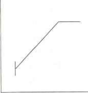
In general, we find the continuous relational form of hypotheses more useful than the categorical "If A, then B" form, for the same reasons that we preferred continuous concepts to categorical ones (see Chapter 2). As we see above, the categorical form "If A, then B" appears to provide less information than the continuous formHypothesis: The more education a person has, the more he or she reads a daily newspaper.

Operational definition for education: The number of years of formal schooling a person has.

Operational definition for newspaper readership: The number of days per week that a person inputs and processes information from a newspaper.

7

0

0 24

Years of education

D ays per week read a daily newspaper

"The more A, the more B." In fact, the operationalization of the concepts in the hypothesis defines whether the hypothesis is continuous or categorical.

Simply put, there are three combinations of categorical and contin­uous variables that yield three types of hypotheses:

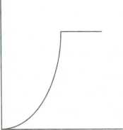
1. Both variables are continuous. "The more people read a newspaper, the more interested they are in politics." The converse could also be supported because causal direction is ambiguous in this relationship. The hypothesis could also be phrased: "There is a positive relationship between political interest and newspaper reading." Figure 3.1 shows the relationship between individuals' education and how frequently they read a newspaper. Both variables are continuous, allowing us to show what a hypothesized straight-line relationship would look like. The slope of the line is arbitrary, but, as we will learn in Chapter 4, the slope should approximate what the theory predicts.

2. One variable is categorical and one continuous. "Women vote more often than men do." Biological sex is assumed to be the independent variable, with number of elections voted in being dependent. This is a

Hypothesis: People with a high level of education read the newspaper more than people with a low level of education.

Operational definition for education: The distribution in Table 3.1 (number of years of formal schooling) is dichotomized into high and low categories by splitting the distribution at the median. (Note: This is done for purposes of illustration only. In general, if you had a ratio-level operational definition, you would not want to dichotomize it. You would lose a substantial amount of information.)

Operational definition for newspaper readership: The number of days per week that a person inputs and processes information from a newspaper.

Й S.

м S

<D Oh

СЛ £ £ ч £

о с

О. ^

СЛ ГД Л

оз ТЗ О оЗ

Low

H igh

Education

classic f-test statistic situation, with sex as the grouping variable and voting as the variable on which means are calculated for each value of sex. Figure 3.2 shows the same sort of relationship if we dichotomize education. The height of the columns is arbitrary but should approximate what the hypothesis predicts.

Although we often think of the grouping variable in a t test as being the independent variable, there are also hypotheses involving categorical and continuous variables in which causal direction is either ambiguous or not intended: for example, "Clinton supporters are younger than Bush supporters are." This hypothesis could certainly be tested with a t test, with candidate as the dichotomous grouping variable and age as the variable on which means are calculated. However, there is no implication that changing the candidate whom a person supports willchange that person's age. Rather, the hypothesis is merely testing the difference in ages between the two groups. As always, making assump­tions about causal direction is difficult and fraught with danger.

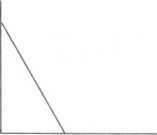
3. Both variables are categorical: "People with less education read the newspaper less [than people with more education]." As is often the case when dealing with categorical variables, not all values of the variables are always included in the hypothesis. Implicit is a continuation of the hypothesis: "than people with more education." Two categorical variables may easily be analyzed with a contingency (cross-tabulation) table, with the presumed cause (in this case, politi­cal party) being the column variable and the presumed effect the row variable. Making the presumed cause or independent variable the column variable is a scientific convention only, but it is one that readers have come to expect. The interpretation of a table will be based on an assumption that this format is being used. Figure 3.3 further dichotomizes newspaper reading into high and low categories, producing a 2 x 2 contingency table. The number of Xs is intended to be an example of the number of people who would fall in each cell, according to the hypothesis.

In the next chapter, we will discuss operational linkages and learn more about how these hypotheses may be represented visually. One form of the operational definition is the graph, as in Figures 3.1 to 3.3.

• CAUSAL DIRECTION

In the first type of hypothesis defined above, to say, "If A happens, then В will happen," implies that A is the cause and В the effect. The same is true of "The more A, the more B." The assumption is that the first variable named is independent.

In cases when it is impossible or unwise to infer causal direction, scholars may wish to substitute the form "A is [positively or nega­tively] related to B." This states the fact of the relationship and the direction of the relationship but does not imply causal direction. However, scholars should not use this more ambiguous relational form merely to avoid making statements that support their convictions. There are ways to argue causal direction that should be used between variables that are related. We caution scholars against using this form merely to avoid the task of establishing causal direction.Hypothesis: People with less education tend to read the newspaper less [than people with more education], (The part in brackets is implied, whether or not explicitly stated.)

Operational definition for education: The distribution in Table 3.1 (number of years of formal schooling) is dichotomized into high and low categories by splitting the distribution at the median. (Note: This is done for purposes of illustration only. In general, if you had a ratio-level operational definition, you would not want to dichotomize it. You would lose a substantial amount of information.)

Operational definition for newspaper readership: Take the distribution shown in Table 3.1 (days per week read a daily newspaper) and dichotomize it at the median. (Note: This is done for purposes of illustration only. In general, if you had a ratio-level operational definition, you would not want to dichotomize it. You would lose a substantial amount of information.)

Low

Newspaper

reading

E ducation Low High

xxxxxx	XXX
xxxxxx
xxxxxx
	xxxxx
	\xxxxx
xxxx
XX

High

Causal direction may be supported in four ways:

The hypothesis must show statistical support for covariation (i.e., a relationship) between the two variables: As one variable changes its values, the other's values also change. Change can be in either a positive or a negative direction. In a positive relationship, the values of one variable change in the same direction as the values of the other. In a negative relationship, the values of the variables change in opposite directions.The presumed cause should occur in time before the presumed effect. This is easy to establish in experiments, where the researcher has control over the timing of administering treatment variables to the subjects. In other research, such as cross-sectional surveys, however, it may be impossible to empirically establish time order, making causality more difficult to establish.

1. The researcher should rule out possible alternative explanations for the observed relationship. In an experiment, if subjects are randomly assigned to treatment groups, random assignment theoretically rules out variance due to an infinite number of unidentified and unmea­sured variables. In surveys, however, researchers must use the litera­ture to identify plausible variables that may be alternative explanations and then find ways to measure them and statistically control for them. The survey researcher's task is more difficult but not impossible. The same constraints apply to content analysis.

2. All researchers must minimize error variance. This may be as simple as ensuring that no errors are made in the study—that all subjects get the designated stimulus, that all respondents are given the same question in the same tone of voice. In practice, however, errors creep in and are inevitable in research. The researcher's job is to mini­mize them. Another form of minimizing error variance is controlling for important variables that are related to the dependent variable. In analysis-of-variance terms, this means keeping the error term of the equation as small as possible. The error term may include variability in the dependent variable not measured by the independent and control variables used in the study. The larger the error term, the less likely statistical significance is to be achieved.

• HOW RESEARCH QUESTIONS AND HYPOTHESES DIFFER

The appropriate use of hypotheses and research questions lies pri­marily in whether one is engaged in deductive or inductive research. The deductive model of science begins with theory, forms hypotheses, collects data to test the hypotheses, and then if necessary revises the theory. Inductive research begins with the data. It forms generaliza­tions that become theory and may be later tested deductively. Although deductive research is ideal to test theories, inductive research is better at building theory.

Research questions are most appropriate in new areas of research in which little is known about the relationships among variables and in which there is scant literature that is applicable. Otherwise, hypotheses should be stated. With the explosion of social science research in recent decades, it is difficult to imagine a study proposal unrelated to any line of previous research. Although the topic may be new, as in the case of a new technology, there have been numerous studies about how people and society relate to new technologies, and surely these can suggest hypotheses for testing. Researchers should not avoid framing hypothe­ses merely because they are not sure whether they will be supported. Sometimes it is even more important to know that a hypothesis is not supported than that it is.

Research questions should be used only when there is a legitimate need for inductive theorizing. They should never be a substitute for a wide-ranging literature search and critical thinking on the part of the scholar. For example, "Does the nature of the protagonist affect how aggressive children are when they see televised violence?" is one or more hypotheses in disguise. The scholar should tap into the literature dealing with identification, fantasy versus reality of presentation, and so on, to form one or more hypotheses about this topic.

The primary danger with research questions is that the "answers" to the questions are often interpreted in the same way as hypothesis results. Yet hypotheses are interpreted narrowly. For example, in response to the question "Is there a difference between the amount that women and men read a newspaper?" it is certainly possible to observe that one mean is bigger than another. Let's say we observe that women read newspapers more frequently. The researcher confidently reports the findings and confirms that women are more frequent readers than men are. Unfortunately, the only thing established is that in the sample men read more than women did. But this is uninteresting information, for the purpose of most research (where less than the population is being studied) is to say something about the population, not about those individuals who by chance were included in the sample.

The same would be true if the means showed that men read news­papers more frequently. All we have established is that in this sample the means are as reported. But some researchers using research ques­tions as confidently report one outcome as the other.

By contrast, the testing of a hypothesis requires that a direction be predicted. We look at the literature and find that in most studies men read newspapers more than women do. Thus, we frame the hypothesis "Men read newspapers more frequently than women do." Instead of using "eyeball statistics"2 to answer the research question, we conduct a t test. The t test gives us the advantage of knowing whether the observed difference between the means is large enough to represent (at some specified probability level) a real difference between the groups in the population or whether the difference is merely due to chance or random error.

Let's say the t test does support the hypothesis and, as in the research question, we conclude that men read newspapers more than women do. Statistical significance in the t test implies that in the popu­lation men read newspapers more than women do, not that this is true just of the sample. This is a major advantage over the eyeball statistics used in the study with the research question.

But what if the results of the hypothesis test are different? What if the hypothesis is not supported? What if there is no difference between men's and women's reading, if women read a lot more, or if men read only slightly more? All three of these would result in lack of support for the hypothesis that men read more than women do. Does this mean that we can conclude that women read more than men do? Definitely not. The logic behind hypothesis tests requires that only statistically significant results in the direction of the hypothesis may be taken as sup­porting the hypothesis. All other results are ambiguous. Did we make a mistake in the study? Was the literature wrong? Further research may be necessary. Null results from a hypothesis test do not necessarily mean that the underlying theory is incorrect; there are many ways in which error may creep into studies, and to give the theory a fair test, the researcher must reconduct the study using different methods.

One last word about research questions: The scholar who poses research questions and then uses inferential statistics (such as the t test) to answer them is committing an error of logic. Inferential statistics are for testing hypotheses, and the researcher should reformulate the research questions as hypotheses.

• NOTES

1. Statistics books distinguish between null and research hypotheses. The null hypothesis is a statement of no difference between the values of a variable or no relationship between variables. Technically, the null hypothesis is tested by statistics. The research hypothesis states the opposite, but it is generally reported in research accounts. Statistical significance implies that the null hypothesis may be rejected and that there is a certain probability that the predictions of the research hypothesis can be generalized from the sample to the population. In this book, the term hypothesis can be assumed to mean the research hypothesis.

2. We use the term eyeball statistics to indicate instances where a researcher looks at, for example, the difference between two means and says, "Well, it looks like Mean A is bigger than Mean B." But how big is big? How big a difference is enough to say something meaningful? Inferential statistics are always better than eyeball statistics, even if the two yield the same result. Inferential statistics allow us to estimate the probability of our being wrong when we say the two means are different. Eyeball statistics rely on a wing and a prayer.

4

Theoretical and Operational Linkages

n

_O

ce hypotheses are formed, it is necessary to specify two sorts of linkages, connections among the variables in the hypothesis. There are two ways of thinking about such connections: First, we demonstrate why each hypothesis or research question ought to be true—that is, why the concepts ought to be related in the way the hypothesis says they are. This is the theoretical linkage. Second, we show how the concepts are related empirically. This is the operational linkage. Both are necessary if the theory is to be fully elaborated.

Theoretical and operational linkages are also necessary for propo­sitions. The theoretical linkage explains why the proposition should be true, without concern about relations among concepts. The operational linkage shows the type of data that support the proposition.

Likewise, for research questions, theoretical linkages explain the logic of the question and justify asking it. The theoretical linkage may provide hypothesized explanations for varying (and perhaps contra­dictory) outcomes or answers to the question.

For assumptions, which are not empirically tested, only theoretical linkages are necessary. However, if the assumption is relational, it may be advantageous to specify some elements of the operational linkage.

• THEORETICAL LINKAGES

The theoretical linkage gives the theory explanatory power. It explains why the hypotheses, assumptions, and propositions should be true, using at least one of three methods. First, one can cite an existing theory and all of the explanations inherent in the theory. Second, especially if one is working in an area in which theory is not well developed, existing literature can be cited that shows results similar to (or, if one intends to refute a theory, different from) those predicted by the hypothesis. Third, and perhaps most important, researchers must be able to state support for the hypothesis in their own words using their own logic. In fact, it is desirable to state multiple reasons why, logically, the hypothesis should be true. If the researcher cannot state at least one good reason why the hypothesis is true, then the hypothesis is unlikely to receive empirical support.'If the researcher can think of 10 good reasons, then the odds are greater that at least one of them will elaborate an empirically supported hypothesis. Of course, it is most desirable for the researcher to use all three methods of explaining the hypothesis under the same reasoning: existing theory, existing literature, and logical reasoning. The more evidence we can muster to support the hypothesis, the more confident we may be that it will be empirically supported.

By these methods, the explanatory power of the theory is increased. Hypotheses, research questions, and propositions are not thrown care­lessly into the theory (or tested individually without thought) but are instead incorporated into a whole, showing why the concepts in the theoretical statements ought to behave in the way specified. This forces the researcher to specify ahead of statistical tests at least one good reason why the hypothesis ought to be supported. It therefore reduces the probability that the researcher will thoughtlessly create hypotheses merely for the pleasure of doing data analysis or that hypotheses will be tested only to satisfy minimal curiosity. Theoretical statements ought to be created out of a theoretical whole, and their introduction into a study is best accompanied by a strong theoretical linkage.

In fact, the group of theoretical linkages supporting the hypotheses in a study is itself the theory that the researcher presents. From what other source can it come? The existing theories, literature, and logical statements are the support for the hypotheses, and, in combination, are the theory on which the study rests. Thus, the specification of individual theoretical linkages for each theoretical statement is crucial.

In practice, most research articles are written with the literature review and theory specified in advance of the hypotheses. Unfortunately, once the hypotheses are reached, the reader may not follow the author's logic in understanding the derivation of the hypotheses, and the theoretical underpinnings of the hypotheses may not be as clear in the reader's mind as in the author's. Therefore, it is valuable to summarize the theoretical linkages given previously in one or two paragraphs, immediately following each hypothesis. This will ensure that the hypotheses are in fact directly derived from the literature and theory previously presented and that both author and reader are clear about the theoretical underpinnings of the hypotheses. Table 4.1 shows three brief examples of theoretical link­ages. In practice, theoretical linkages should be more complete and elaborated upon.

The examples shown in Table 4.1 illustrate how the three types of theoretical linkage—theory, literature, and logic—can be used together to explain why the hypothesis should be supported. In areas where theory is sparse, or where the scholar is building theory, the specifica­tion of existing theory may be missing, or theories tangentially related to the topic may be mentioned. It is perfectly reasonable to build one's own logical structure to defend hypotheses; this is the creative side of scholarship that should be encouraged.

Although we have been talking about theoretical linkages for hypotheses, propositions and assumptions should also have theoretical linkages. They are especially important in assumptions, where the reader may or may not agree with the assumption after reading the justification for it.

T Creating theoretical linkages for research questions presents a spe­cial case. Because no prediction is made by the research question, the theoretical linkage should not take sides—for example, present a local argument for one particular potential answer over another. However, the authors should know enough about the topic to be able to intelli­gently discuss the possible outcomes. Some literature may predict one outcome and other literature a different outcome. Logical arguments may be made for different outcomes. These sorts of differences should be discussed as the theoretical linkage so that we know the authors are not merely "fishing" for results but rather have thought through the research questions thoroughly and know as much as is knowable about the topic being studied.Hypothesis 1: Concept Names: Theoretical Definition: Operational Definition: he more the media	IV—Amount of media	IV—Amount of media	IV—Number of stories about crime
emphasize an issue,	coverage	coverage is an assessment		Range: 0 to infinity
the more important	DV—Importance of	of the volume of coverage,		DV—	Survey responses to the
people think it is.	issue to the public	or the degree to which a story dominates news coverage overall. DV—Importance of the issue		question "How important is the issue of crime to you?" Responses: 5 = very important-, 4 = important; 3 = neither important
		is the degree to which the		nor	unimportant; 2 = unimportant;
		public believes that the		1 =	very unimportant
		topic is more important
		than other topics in the
		news.
		Theoretical Linkage:		Operational Linkage:
		More coverage of an issue in
		the media will put it more
		prominently in people's		OJ Ё in
		minds. Over time, the focus		b ts 41	/
		by the mass media on an		It И m	s'
		issue, such as the crime rate,		с CC	s'
		will result in more people		о N a, e ~	s'
		identifying that issue as an			s'
		important one (McCombs &		0	"
		Shaw, 1972).		Number of stories about
					crime

(Continued)

H Table 4.1 (Continued) ypothesis 2:	Concept Names:	Theoretical Definition:	Operational Definition:
The more a society is	IV—Level of social	IV—Level of social integration is		IV—	The proportion of the people
integrated through	integration	the degree to which the		who are affiliated with a church
shared norms, the less	DV—Suicide rate	individual members of a social		or other social group (as a
likely it is that its		group feel connected to the		percentage of the total
members will commit		group through shared values		population)
suicide.		and a shared ideology.		Range: 0% to 100%
		DV—Suicide rate is the		DV-	-Per capita rate of self-inflicted
		proportion of people in social		deaths (the rate of self-inflicted
		groups who take their own		deaths per 1,000 people)
		lives.		Range: 0 to 1,000
		Theoretical Linkage:
		Because suicide often is		Operational Linkage:
		precipitated by feelings of
		isolation and loneliness, links		О 0) o
		to a social group through		Is
		shared ideas and beliefs			'Ч
		should reduce a person's		'3 со
		sense of isolation. The		<3 u cC u
		reduced anomie at a societal			N
		level should result in a		J-4 <U C-.
		reduced suicide rate		о
		among that social group			0% 100%
		(Durkheim, 1951).			Proportion of people belonging to church or other social group

(Continued)

Hypothesis 3:

C oncept Names:

T heoretical Definition:

O perational Definition:

The greater an individual's sense of self-efficacy, the more likely it is that he or she will make a lifestyle change to improve his or her health.

IV—Sense of self-efficacy DV—Likelihood of undertaking a healthy lifestyle change

IV—Sense of self-efficacy is the degree to which someone believes that he or she can do what he or she sets out to do.

DV—Likelihood of undertaking healthy lifestyle change is the degree to which someone is likely to modify a current behavior to improve his or her health.

Theoretical Linkage:

A greater sense of self-efficacy, or the ability to succeed at a task or goal, will increase the chances that a person will even attempt a behavior change. Those with low self-efficacy, and who therefore believe they are likely to fail, will see little value in even making the attempt at a healthy behavior change (Bandura, 1997).

IV—Survey responses to the question "How satisfied are you with your level of personal success?"

Responses: 5 = very satisfied;

4 = satisfied; 3 = neither satisfied nor unsatisfied; 2 = unsatisfied; 1 = very unsatisfied DV—Survey responses to "How likely are you to start a new exercise or self-improvement program in the next 3 months?" Responses: 5 = very likely; 4 = likely;

3 = neither likely nor unlikely;

2 = unlikely; 1 = very unlikely Operational Linkage:

Cl

О

-о

та

га

£

■а

Satisfaction with personal success

• OPERATIONAL LINKAGES

Telling how the variables in the hypothesis are related is the job of the operational linkage. Operational linkages may be presented in two forms, visual and statistical. We recommend that researchers, par­ticularly those early in their careers, prepare both sorts of operational linkages. They will take the form of figures and statistical tables.

It is of primary importance that researchers understand that both types of operational linkages must be prepared before any data are collected. If the researchers are able to graphically illustrate what their hypotheses predict and statistically explain how the hypotheses will be tested, then they are more likely to include all variables needed to test the hypotheses. Often researchers who have not clearly thought through their studies collect and analyze their data and then wish that such and such a variable had been included. The graphic and statistical forms of operational definitions make such mistakes highly unlikely.

For beginning scholars who are unfamiliar with statistics, it is at least necessary that they prepare the graphic form of the operational linkage. This requires no knowledge of statistics and helps the researcher think through the potential testing of the hypothesis.

The graphic form of operational linkage is not included in final research projects, which place their emphasis on the degree of statisti­cal support for the hypothesis after data analysis, not on what the hypothesis graphically predicted. On the other hand, research propos­als, such as thesis or dissertation proposals, are often aided by the inclusion of graphic operational linkages because they help not only the researcher but the committee in evaluating whether all elements of the study are present and whether the student is ready to proceed with data collection.

Operational Linkages as Visual Representations

The simplest form of operational linkage is a pictorial representa­tion of the hypothesis. For example, Figure 4.1 shows a simple graphic operational linkage for the hypothesis "The more television violence children view, the more aggressive acts they portray." The horizontal axis is generally taken as the independent variable and designated as x (see Figure 4.2), and the vertical axis is assumed to be the dependent variable, called y.Figure 4.1 A graphic operational linkage for the hypothesis "The more television violence children view, the more aggressive acts they portray"

О

Ы) i—

bJ) 1) й D-

о g

fc I 2

g S =

Exposure to television violence (number of violent TV shows watched)

Figure 4.2 The x and у axes

Generally labeled the у axis, meaning it is the dependent variable

Generally labeled the x axis, meaning it is the independent variable

Figure 4.3 The data are never as neat! The line represents the closest fit to all data points

.0

<D Г73

0. -

Z D.

E xposure to television violence (number of violent TV shows watched)

С Л

О

<D

>

In Figure 4.3, the slanted line is a visual representation of the hypothesis, whereas the dots represent real data collected. Remember, we draw the operational linkage before collecting data. Once we collect data, we will see that the reality of the data do not neatly fit the hypoth­esized line. The difference between our hypothesized relationship and the data expresses how closely our hypothesis is supported.

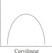
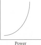
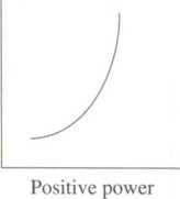
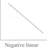
When preparing operational linkages as visual representations, we have four considerations: the form of the relationship (linear, curvilin­ear, or power), the direction in which the variables are related (positive or negative), the coefficients (constant and slope), and the limits (the range within which the hypothesis is supported).1

Form of the Relationship

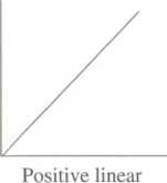
As Figure 4.4 shows, relationships may be hypothesized to be linear, straight lines. In these relationships, one or more units of change in th

eLinear—As the values of one variable increase, the values of the other variable increase (or decrease).

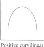
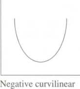
Curvilinear—As the values of one variable increase, the values of the other increase (or decrease) up (or down) to a point and then start off in the other direction.

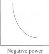
Power—As the values of one variable increase, the values of the other variable increase (or decrease) at an accelerated rate.

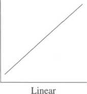
independent variable are accompanied by one or more units of change in the dependent variable, in a precise and constant manner. Such relationships are frequently hypothesized in the social sciences but are rarely seen as pure cases. Reality rarely fits a straight line; however, most statistics test for the presence or absence of a straight-line relation­ship. Thus, this basic relationship is commonly used.

Curvilinear relationships may form the letter "U" in an inverted or upright position, or they may be shallow curves in either direction.

Power curves are a special case of curvilinear relationships, where a change in the independent variable has a huge change in the dependent variable at one point in the relationship. There is very little change in the dependent variable initially, then a huge change, then very little change.

Direction of the Relationship

Here we specify whether the units of a variable change in the same direction (positive) or in opposite directions (negative). In a positive relationship (Figure 4.5), an independent variable's and a dependent variable's values change in the same direction (e.g., both higher). In a negative relationship, they change in opposite directions (e.g., the independent variable increases in its value, whereas the values of the dependent variable decrease in value).

Positive—As the values of one variable increase, the values of the other variable also increase.

Negative—As the values of one variable increase, the values of the other variable decrease

.

The Coefficients

The slope indicates how steep or shallow the line is (Figure 4.6). A steep line indicates that a one-unit change in the independent variable is accompanied by more than one unit change in the dependent variable. A shallow line might indicate that a one-unit change in X is accompa­nied by less than a whole-unit change in Y.

The constant indicates where the line crosses the у axis. This tells us what the value of Y is for what is generally the minimal value of X. (Exceptions occur where, for example, the scale of the independent vari­able ranges from negative to positive values, with zero in the center. The constant would probably be where Y crossed the zero point of X.)2

The Limits

As Figure 4.7 shows, increases in X may not indefinitely be accompanied by increases in Y. Take the example of the hypothesis "The more education a person has, the more he or she will read a daily newspaper."

Constant—The value of the dependent variable (on the у axis) when the line

crosses the у axis.

Slope—Simply, how steep or shallow the line is. Technically, a description of the amount of change that we predict will occur on the у axis when the value on the x axis changes by 1. The larger the coefficient, the more of an effect X has on Y.

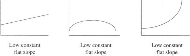
High constant High constant High constant

steep slope steep slope steep slope

A person may have indefinite years of education, but there are only 7 days a week available for newspaper reading. In reality, newspaper reading evens off after a relatively small number of years of education, say high school graduation or some college.

The figure shows boundary limits for linear, curvilinear, and power relationships, but the examples illustrate only some of the possible limits that may be hypothesized.

Operational Linkages as Statistics

Operational linkages are often expressed in statistical terms, such

as a statistically significant and positive Pearson's correlation coefficient.

The limits indicate that the relationship predicted by the hypothesis is supported only within a certain range of its variables' values. Example: The ceiling effect holds that the relationship operates only below a certain threshold

.

This is appropriate for the researcher to specify before the data are collected because it keeps the researcher honest about what types of results will support the hypothesis. In fact, it is desirable as part of the operational linkage for the researcher to prepare tables that specify the statistical analyses to be performed. The tables are incomplete only in that the final numerical statistical results are not provided. Appendix A includes examples of typical tables that may be included as operational linkages. It is advisable to begin with univariate statistics before pro­ceeding to inferential statistics that may begin hypothesis testing. Bivariate and multivariate statistics complete hypothesis testing. Start with the simple and proceed to the complex.

A major advantage of specifying in advance all of the tables that will be included in the statistical analysis is that the researcher will be sure that all variables needed in data analysis are in fact being included. This helps the researcher in conceptualizing the study and in ensuring that all the data needed are in fact being collected.

Appendix A does not include every table or figure that may be needed in a study, but it covers most of the basics. To use the tables in Appendix A, it is necessary to know the level of measurement of each variable in the study. As you will see in Appendix B, levels of mea­surement range from nominal to ordinal, to interval or ratio. Nominal variables use arbitrary numbers to represent the values of the variable. For example, 1 can be assigned as "male" or "female" for the variable gender. The numbers are like names assigned to the values. Nomina

lvariables have the characteristics of being exhaustive (all possible values/categories of the variable are represented) and mutually exclu­sive (an item can be placed only in one value of the variable). Ordinal variables include the characteristics exhaustiveness and mutual exclu­sivity, as well as order. That is, the numbers assigned to the values must be in a numerical and meaningful order. For example, a variable with high, medium, and low values could have them assigned as 3, 2, and 1, respectively. We cannot logically assign them as 2, 3, and 1, for the order of the numbers would not be the same as the order of the values. Interval variables include the characteristics of exhaustiveness, mutual exclusivity, and order, as well as having equal intervals between the numbers and their values. For example, the Celsius temperature scale assigns 100 to the boiling point of water and 0 to its freezing point. These assignments of numbers to these variables are arbitrary once order is achieved, but the scale's values are equally spaced between 0 and 100. A temperature of 80 is twice as hot as a temperature of 40. The amount of heat gained when moving from a temperature of 10 to 11 is the same as moving from 39 to 40.3 Ratio variables have all of the characteristics of nominal, ordinal, and interval variables, as well as having an absolute zero. In the other three levels, zero can be assigned to any value arbitrarily. In ratio variables, zero can only mean none of the concept. For example, in the Kelvin temperature scale, zero represents no heat.

• THE WHOLE STORY

The specification of the operational linkage puts all of the parts of the theory together, and the theory may be shown in brief in Table 4.1. This brings together all of the parts we have been talking about in Chapters

2. 3, and 4. Although none of the three theories mentioned in Table 4.1 is complete, the table does suggest how complete theories may be elaborated. A completely elaborated theory would include all assump­tions and hypotheses used, their concepts, and their definitions and linkages. This is an overwhelming task, but one that would help advance social science by making theories much more explicit than they are today and would therefore allow scholars to test the theories and advance them through support, modification, or lack of support. The current state of social science theories is much more vague, with one scholar meaning one thing by a concept and another scholar meaning something else entirely. Once definitions and linkages are specified explicitly, a base will have been established that will permit the growth of theories. Connections among theories may be made more easily, and the state of social science research will advance more quickly and with logical deliberation.

• NOTES

1. The following is adapted from Hage (1972), pp. 85-110.

2. The terms constant and slope are familiar to those who know regression statistics, but knowledge of this statistical procedure is not necessary to conceptually understand these terms.

There are occasional disagreements over what is interval and what is ordinal. For example, the Likert scale ( 5 = strongly agree, 4 = agree, 3 = neutral, 2 = disagree, 1 = strongly disagree) is treated by some social scientists as an inter­val scale, using the logic that values represent equal-appearing intervals: That is, people interpret the intervals as being equal. Others are more conservative and use this as an ordinal scale.

5

Theoretical Statements Relating Three Variables

_A

frequent occurrence in communication research is to begin a line of inquiry with a hypothesis of broad, across-the-board effects, only to find in subsequent research that the effect is not general but occurs only under certain conditions. What started out as a clean, neat two-variable hypothesis needs to be qualified. The hypothesis is no longer parsimonious; it needs to have qualifying phrases tacked on. And it is no longer as general, and therefore not as potent; it holds up only in certain situations. Meadow (1985) appeared to have been referring to this occurrence when he wrote, "After four decades of exploration, we are left with one answer to the question of media effects—'it depends'" (p. 158).

Faced with this kind of outcome, we can easily imagine a process with no end. Will further research uncover still more qualifying vari­ables, until it takes knowledge of 50 variables to make a prediction and only a computer can handle the complexity?

Meadow is right, of course, but his conclusion should not be the basis for throwing up our hands in despair. In fact, another point of view is that this is just the place at which things get interesting. As we find out more about the details of these dependencies, we are finding out something about the complexities of human behavior and the variables that make a difference. The proof of the pudding is that knowl­edge of the dependencies or the contingent conditions often lets us make more accurate predictions about social interactions and other forms of human behavior. In short, there's a big difference between saying, "It depends, but I don't have any idea on what" and "It depends, and the two or three most important variables it depends on are X, Y and Z."

Part of the solution to this dilemma may lie, as it often does, in taking a middle course. On the one hand, two-variable relationships are probably too simplistic. On the other hand, 50-variable relationships are probably too complicated. Even a path model with just five variables can be so complex that it is difficult to understand. But fortunately there is a range of possibilities in between these. What might make sense as a research strategy in many areas is to explore three-variable relation­ships, the next level of complexity beyond two-variable relationships. As we shall see, this next step increases the complexity quite a bit. And it seems like a natural step in that it takes us beyond Hage (1972), whose valuable book deals mostly with two-variable relationships.

Further, it may not be necessary to study a huge number of variables all at once. As Hirschi and Selvin (1967) noted, "The increasing success of the life sciences in understanding the human body (surely more highly integrated than the social system) suggests that good research is possible without taking everything into account at once" (p. 22).

This chapter discusses the next step in theory building in the social sciences beyond the formulation and testing of two-variable hypotheses. As Eveland (1997) noted, "Many theories ... in mass communication and related fields predict more complex effects than the simple linear and additive effect of independent variables" (p. 405).

For instance, the knowledge gap hypothesis suggested by Tichenor, Donohue, and Olien (1970), which has generated a great deal of subse­quent research, is basically a three-variable relationship. A graph illus­trating the knowledge gap hypothesis is presented in Figure 5.1. The graph shows a relationship between exposure to information and knowledge, with knowledge increasing as exposure to information increases. But it also shows that the rate of increase in knowledge is different depending on the socioeconomic status of the individual. This kind of three-variable relationship is called an interaction. We have an interaction when the relationship between one variable and a second variable is different depending on the values of a third variable.High socio-economic status

6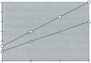

5

4

Knowledge 3 2 1 0

2 3

Time (or exposure to information)

• L ow socio-economic status

Hage's (1972) book focused on two-variable theoretical statements, for which he recommended the form "The greater the X, the greater the Y." He acknowledged the importance of relationships that are more complicated than two-variable relationships, but he didn't do very much to deal with them. He wrote:

Through our discussion, we have been concentrating on the prob­lem of interrelating just two variables. In practice, we can and do expect our operational linkages to be more complex than this. The diagrams and forms refer to the effect of X on some Y where X can be a combination of variables, (p. 109)

The idea that X can be a combination of variables oversimplifies the complexity of even a three-variable relationship quite a bit. As we shall see, a set of three variables can be related in five distinctive ways. The situation becomes even more complicated with more than three variables.

Of course, it is a common research strategy to introduce a third variable as a control variable while exploring a relationship. The usual reason for doing this is to test whether a relationship is spurious. This is indeed an important reason for introducing a third variable. Actually, however, there are at least three other important roles that exploring three-variable relationships can play in the development of theory.ROLES OF THREE-VARIABLE RELATIONSHIPS IN THEORY

One of these important roles is specifying the ways that a hypothesis expressing a relationship between two variables either holds up or does not hold up depending on the state of a third variable. This is sometimes spoken of as specifying the "contingent conditions" (Winter, 1981, p. 236) or as exploring "contingent causation" (Chaffee, 1977, p. 226). As Chaffee noted,

Physically partitioning samples on the basis of contingent orienta­tions that are necessary for a media effect to operate is likely to become more common in future research; this trend is a sign both that we understand quite a bit about the total influence process and that we are going to be able to learn more. (p. 227)

An example of research that specified contingent conditions for com­munications effects to take place is Hill's (1985) study of agenda setting by television news. He found that agenda-setting effects are more likely when viewers have prior awareness of news topics through print media exposure or have some college education.

A second major role that exploring three-variable relationships can play in building theory is in clarifying causal relationships by showing the operation of intervening variables. This is the process of analysis that Hyman (1955) called interpretation. Commenting on the area of mass media effects research, Chaffee (1977) stated, "What has been lacking, although it too is beginning to accumulate, is three-variable research in which the psychological processes that intervene between media exposure and its effects are studied" (p. 222).

Chaffee (1977) gave an example of a research area where there is a need for interpretation. He cited the finding that a boy is shown a filmed fight and subsequently acts more aggressively than before. We might conclude that the film has had an effect, but we might not under­stand the intervening psychological process that led to this effect. In this example, there are several possible intervening processes—the boy may be imitating the behavior he has seen; the boy may be "identify­ing" with the grown, strong man who was fighting; or the film may have aroused him to do something physically active, and any kind of activity may have reduced that state of arousal. We don't know which of these possible interpretations is correct until we do some additional three-variable studies.

To take another example, interpretation could be useful in clarifying our understanding of how agenda setting works. We don't really know much about the process by which the play of news items in the media gets translated into a set of priorities in an individual's mind. One pos­sibility—and this is only one of many—is that the public has a good understanding of journalism and interprets the cues of news play as indicators of importance. We could test this possibility by introducing as a third variable a new concept called journalistic savvy. This variable would attempt to measure understanding of the various journalism conventions used to indicate story importance. This variable could be measured by having survey respondents indicate their agreement on 5-point Likert scales with statements such as the following:

"If a news story is on the front page of a newspaper, it is important."

"The most important stories in a television newscast come at the beginning of the newscast."

"The larger the photograph that accompanies a story, the more important the story."

Once these kinds of variables have been measured in an agenda-setting study, they can be used as third variables in the kind of three-variable analysis we are recommending.

There are many other good candidates for variables that would help us understand the agenda-setting process by using a third variable to interpret the two-variable agenda-setting relationship. An excellent way to focus one's theory-building efforts is to think of possible variables of this type, figure out how to measure them, and then conduct a study in which they can be introduced as third variables along with the two principal variables of the agenda-setting process (the media's agenda and the public's agenda).

A third important reason for exploring three-variable relationships is that it can help specify the operating component of a global variable (Rosenberg, 1968). For instance, a researcher may find that whether people vote is related to social class. But social class is a global variable with a number of components, including education, income, social pres­tige, and type of occupation. Which component (or components) of social class is operating to influence voting behavior? Bringing each component variable into a three-variable analysis with social class and voting can help to pinpoint the active variable and in doing so will sharpen our understanding of the causes of voting or not voting.

• FIVE TYPES OF OUTCOMES

We have been focusing on a general research strategy in which two vari­ables are cross-tabulated and then a third variable is introduced as a control or test variable. This strategy has been referred to as elaboration by Paul Lazarsfeld (1955a), who did much of the work to develop it. The elaboration model was first described in a paper that Lazarsfeld pre­sented to the American Sociological Society in 1946. That paper was not published in a journal because "at that time, there was little interest in methodological discussion" (Lazarsfeld, Pasanella, & Rosenberg, 1972, p. 125). The model was first presented in published form by Patricia L. Kendall and Lazarsfeld (1950), and the original Lazarsfeld paper was finally published in 1955 (Lazarsfeld, 1955b). The strategy of elaboration research is discussed in Hyman's (1955) Survey Design and Analysis and Rosenberg's (1968) Logic of Survey Analysis.

Lazarsfeld (1955a) and Hirschi and Selvin (1967) indicated that there are four possible outcomes of this type of analysis. But there appear to be five significant ones.

In the following discussion of this kind of analysis, the terms independent variable and dependent variable will be used, even though the variables are not necessarily being manipulated in an experiment. Independent variable will be used to refer to the variable thought to be the causal variable. Dependent variable will be used to refer to the variable thought to be caused, or to be the effect. Control variable or test variable will be used to refer to the third variable brought into an expanded analysis of a two-variable relationship. An intervening vari­able is "one that is viewed as a consequence of the independent variable and a determinant of the dependent variable" (Rosenberg, 1968, p. 54).

1. Explanation. Explanation is one of the possible outcomes of three- variable analysis discussed by Hyman (1972). Explanation occurs when the third variable is causally prior to the independent variable and accounts for the original relationship (see Figures 5.2a, 5.2b, and 5.2c). In this situation, we conclude that the original relation­ship was spurious, and we discard the original relationship. This is not a total loss, however, because we have learned something about the causal relationship. We have learned that the third variable is a more plausible cause of the dependent variable than the original independent variable.

Figure 5.2a Single people appear to eat more candy than married people do. Is this relationship genuine, or is it spurious?

	100
	90
	80
	70
Percent	60
eating
candy	50
regularly
	40
	30
	20
	10
	0

Single

M arried

S OURCE: Adapted from Hans Zeisel (1968), Say It With Figures, 5th ed. New York: Harper & Row, p. 139.

Figure 5.2b We control for age and find that younger people eat more candy than older people, but there is no real difference between single and married people's candy eating. This is a case of explanation—we have found that age is an alternative (and better) explanation for the original relationship.

25 years old i 25 years

Single

Figure 5.2c A line graph also shows that marital status is not related to

eating candy, once we control for age. The lines are essentially parallel.

2. Internal Replication. This term appears to have been introduced by Hirschi and Selvin (1967). Internal replication occurs when the third variable does not affect the original relationship (see Figures 5.3a, 5.3b, and 5.3c). In this case, we conclude that the third variable is not an important variable in this relationship. Our faith in the original two-variable relationship becomes strengthened because we have ruled out one possible alternative hypothesis.

Figure 5.3a It appears that heavy TV viewers are more likely to give the TV answer to a survey question than light viewers are. But will this relationship hold up once control variables are introduced?

8

100 т ; - - • --

90 -• '■ ‘ ;

0 '»«■ I ' lit I Г rfKlLfcit