3. Fir filter design via weighting method.

The useful signal x₁ is accompanied with a white noise x₂ whose intensity is equal to A_sh. For odd variants x₁=A_s·sin(2πt/T) and for even variants x₁=A_s·cos(2πt/T). It is known the order of the filter and sampling time T_s. It is necessary:

1. to plot useful signal x₁;

2. to generate white noise x₂ with intensity A_sh;

3. to plot white noise x₂;

4. to calculate and plot noisy signal x;

5. to calculate cut-off frequency;

6. to design two low-pass filter with given windows;

7. to plot impulse and frequency response of the designed filters;

8. to perform filtration of noisy signal x by means of both filter and filtfilt operators.

To define a cut-off frequency it is necessary perform normalization procedure. LPF normalized frequency is defined as follows

.

Let us define normalized frequency ω_n for Variant 7. According to initial data T=0.001 s and T_c=5 s. thus, normalized frequency is defined as

Variant 1

Rectangular and Hamming windows.

t=20 sec; A_s=0.75; T=1 sec; A_sh=0.3; T_s=0.01 sec; N=10.

Variant 2

Rectangular and Hamming windows.

t=15 sec; A_s=5; T=10 sec; A_sh=0.9; T_s=0.005 sec; N=30.

Variant 3

Rectangular and Blackman windows.

t=30 sec; A_s=1; T=2 sec; A_sh=0.4; T_s=0.01 sec; N=16.

Variant 4

Rectangular and Blackman windows.

t=25 sec; A_s=7; T=10 sec; A_sh=1; T_s=0.001 sec; N=40.

Variant 5

Rectangular and Hamming windows.

t=10 sec; A_s=1.5; T=2 sec; A_sh=0.2; T_s=0.001 sec; N=20.

Variant 6

Rectangular and Hamming windows.

t=30 sec; A_s=7; T=20 sec; A_sh=1.2; T_s=0.003 sec; N=40.

Variant 7

Rectangular and Blackman windows.

t=20 sec; A_s=3; T=5 sec; A_sh=0.4; T_s=0.001 sec; N=20.

Variant 8

Rectangular and Blackman windows.

t=25 sec; A_s=11; T=30 sec; A_sh=1.5; T_s=0.007 sec; N=120.

Variant 9

Rectangular and Hamming windows.

t=25 sec; A_s=5; T=8 sec; A_sh=0.7; T_s=0.005 sec; N=30.

Variant 10

Rectangular and Blackman windows.

t=20 sec; A_s=0.5; T=20 sec; A_sh=0.1; T_s=0.002 sec; N=60.

Example 3

Let us consider a procedure of low pass Butterworth filter design that meets the following performance requirements: Hz, Hz, maximum pass band ripples, , dB, stop band ripples , dB. By defining filter specification within Digital Filter Design Block parameters, we obtain the Butterworth LPF of the order, n=1. The result of appropriate filter functioning is given in Fig.8. The filter zeros and poles location is given in Fig.9.

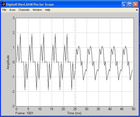
Figure 8 Simulation results

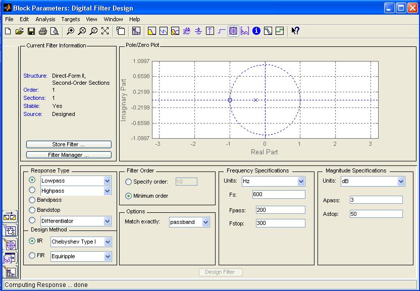
Figure 9 Filter Zero-Pole Plot