

LABORATORY WORK № 8
DIGITAL FILTERT DESIGN
BRIEF THEORETICAL INFORMATION
The Goal of Filtration and Types of the Filters
In order to receive the useful signal on the basis of given sampled signal it is necessary to calculate and design a device (a program for personal computer) realized such transformations of sampled input that distortions caused by noises will be minimized on its (device) output. Such device is called a filter.
The goal of filter design is the ensuring of frequency-dependent modification of given sequence of data (signal). In the simplest case the goal of low pass filter design is the building of the link which would guarantee of absence of attenuation disturbance of input signal in frequency domain from 0 to some given frequency and efficient suppression of harmonic components with more high frequencies.
An analog filter can be represented with continuous transfer function
![]() ,
,
where
![]() and
and
![]() are Laplace transform of input and output filter signals
correspondingly.
are Laplace transform of input and output filter signals
correspondingly.
Digital Filters: FIR Digital Filters
A digital filter is a basic building block in any Digital Signal Processing (DSP) system. The frequency response of the filter depends on the value of its coefficients, or taps. Many software programs can compute the values of the coefficients based on the desired frequency response.
Digital filters are usually classified by duration of their impulse response, which can be finite or infinite. The methods for designing these two filters classes differ considerably.
In general, the z-transform Y(z) of a digital filter’s output is related to the z-transform X(z) of the input by
![]() , (1)
, (1)
where H(z) is the filter’s transfer function. Here, the constants bi and ai are the filter coefficients and the order of the filter is the maximum of n and m.
A Finite Impulse Response (FIR) digital filter is one whose impulse response is of finite duration (i.e. filters whose response to unit impulse (unit sample function) is finite in duration).
The general difference equation for a FIR digital filter is
![]() , (2)
, (2)
where
![]() is the system’s impulse response,
is the system’s impulse response,
or by applying eq. (1) the transfer function for FIR filter can be represented as follows
![]() and
and
![]() .
.
Note that the FIR filter output depends only on the previous N inputs. This feature is why the impulse response for a FIR filter is finite.
Advantages of FIR Filters
FIR filters are simple to design and they are guaranteed to be bounded input-bounded output (BIBO) stable. By designing the filter taps to be symmetrical about the center tap position, a FIR filter can be guaranteed to have linear phase. This is a desirable property for many applications such as music and video processing. FIR filters also have a low sensitivity to filter coefficient quantization errors. This is an important property to have when implementing a filter on a DSP processor or on an integrated circuit.
The primary disadvantage of FIR filters is that they often require much higher filter order than IIR filters to achieve given level of performance.
FIR filters are described by one vector b only. The denominator of their discrete transfer function is identically equal to 1.
The group of functions fir1 is intended for calculation of coefficients b of digital FIR filter with linear phase by weighting method via window functions.
General form of this command is given below.
[b,a]=fir1(n,Wn, ‘ftype’, window).
This command calculates the coefficient vector b of FIR filter with normalized cut-off frequency.
The parameter ‘ftype’ sets the desirable type of the filter (low pass, high pass, band pass or stop band filter).
The parameter window allows set the type of window. If this parameter is not specified than Hamming window will be by default.
Example 1 Create 10-nth order digital low pass filter with normalized cut-off frequency Wn=0.6, using Hamming window.
Matlab code:
L=n+1; % n is an order of the filter
win=hamming(L);
[b,a]=fir1(10,0.6,'low',win);
b= 0.0000 0.0127 -0.0248 -0.0638 0.2760 0.5997
0.2760 -0.0638 -0.0248 0.0127 0.0000
a=1.
The Impulse and Frequency Responses of Digital Filters
The impulse response of the filter with numerator coefficients b and denominator coefficients a is calculated by means of operator impz.
Its syntax is
Impz(b,a)
The frequency response of the filter with numerator coefficients b and denominator coefficients a is calculated by means of operator freqz.
Its syntax is
freqz(b,a)
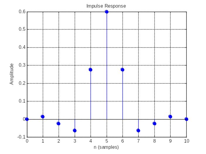
Example 2 Plot the impulse and frequency response of the 10-nth order digital low-pass filter obtained in example 1.
Impz(b,a)
freqz(b,a)
Received plots are shown below.

Filtering Data in Matlab
Filtration is realized in Matlab by means of the operator filter. Its syntax is the following
y=filter(b,a,x),
where x is given vector of input values, y is a vector of filter output values.
Iir Digital Filters
Another type of digital filter is the Infinite Impulse Response (IIR) filter. The impulse response of an IIR filter is of infinite duration. The general difference equation for an IIR digital filter is
![]()
Note that, unlike the FIR filter, the output of an IIR filter depends on both the previous N inputs and the previous M outputs. This feedback mechanism is inherent in any IIR structure. It is responsible for the infinite duration of the impulse response.
Iir Digital Filters Design
IIR filters are digital filters with infinite impulse response. Unlike FIR filters, they have the feedback (a recursive part of a filter) and are known as recursive digital filters therefore. There is one problem known as a potential instability that is typical of IIR filters only. FIR filters do not have such a problem as they do not have the feedback. For this reason, it is always necessary to check after the design process whether the resulting IIR filter is stable or not.
IIR filters can be designed using different methods. One of the most commonly used is via the reference analog prototype filter. This method is the best for designing all standard types of filters such as low-pass, high-pass, band-pass and band-stop filters.
There are three main methods for converting an analog filter into a digital filter:
Impulse invariant method;
Backward difference method;
Bilinear transformation (also known as Tustin’s transformation).
Iir Design Steps:
specify properties of the desired system (tolerance scheme);
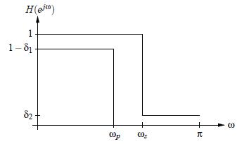
Figure 1 Analog filter tolerance scheme
transform tolerance scheme into tolerance scheme of an analog filter;
design analog filter;
transform analog filter into discrete – time filter.
Impulse Invariant Method
In general poles are mapped as
![]() ,
T is the sampling period.
,
T is the sampling period.
Since any rational transfer function with numerator degree strictly less than the denominator degree can be decomposed into partial fractions as follows
 .
.
Since poles are mapped as stable analogue filter is transformed into stable digital filter
![]() ,
,
![]() .
.
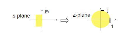
Figure 2 Impulse Invariance Method poles transformation
Advantage: preserves the order and the stability of the analog filter.
Disadvantage: Not applicable to all filter types (high pass, band stop);
There is distortion of the shape of frequency response due to aliasing.
Backward Difference Method
The analog-domain variable s represents differentiation. We can try to replace s by approximating differentiation operator in the digital domain:
 .
.
Thus,
 ,
,
![]() ,
,
 ,
T
is the sampling interval
,
T
is the sampling interval
which suggests the s-to-z transformation
 .
.
Let us consider the second order derivative
 This
means that
This
means that
 .
.
Similarly, one can easily check by induction that
 .
.
Thus, to convert the analogue filter into a digital one, we simply use
![]() ,
a=analog
transfer function.
,
a=analog
transfer function.
![]() .
.
|
|
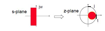
Figure 3 Backward Difference Method poles transformation
Stable analogue filters are mapped into stable digital filters, but pole location for digital filter confined to only a small region (No high pass filter possible!).
Bilinear Transform
Mapping that transforms (whole!) jω-axis of the s-plane into unit circle in the z-plane only once i.e. that avoids aliasing of frequency components.
![]() .
.
|
|
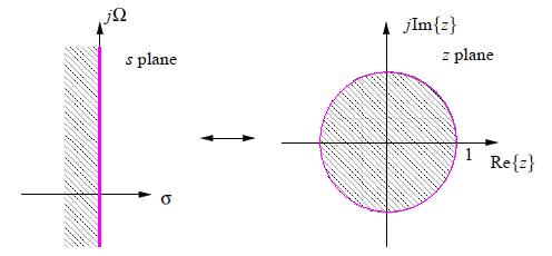

Figure 4 Bilinear Method poles transformation
Frequency
axis of the continuous-time filter: s=jΩ ![]()
Frequency
axis of the discrete-time filter: z=exp(jω) ![]()
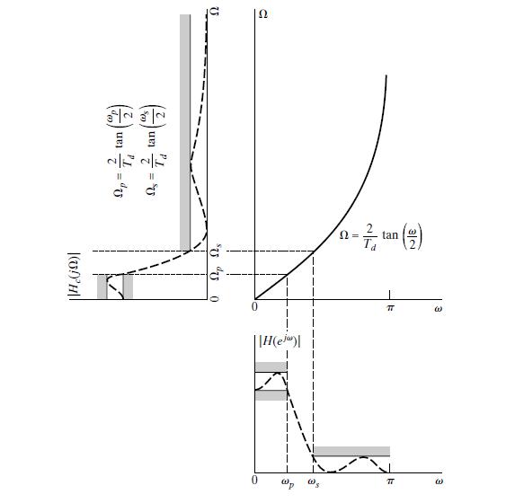
Figure 5 Frequency warping inherent in the bilinear transformation of a continuous-time lowpass filter into a discrete-time lowpass filter. To achieve the desired discrete-time cut-off frequencies, the continuous –time frequencies must be pre-warped as indicated
Thus, bilinear transform maps the LHP s-plane onto the interior of the unit circle in the z-plane. This property allows us obtain a suitable frequency response for the digital filter, and also to ensure the stability of the digital filter. The bilinear transformation avoids the problem of aliasing because it maps the entire imaginary axis of the s-plane onto the unit circle in the z-plane. The price paid for this, however, is the nonlinear compression the frequency axis (warping).
Advantages of IIR Filters
IIR filters are useful for a high-speed design because they typically require a lower number of multiplies compared to FIR filters. IIR filters can also be designed to have a frequency response that is a discrete version of the frequency response of an analog filter. Unfortunately, IIR filters do not have linear phase and they can be unstable if not designed properly. IIR filters also are very sensitive to filter coefficient quantization errors that occur due to using a finite number of bits to represent the filter coefficients. One way to reduce this sensitivity is to use a cascaded design. That is, the IIR filter is implemented as a series of lower-order IIR filters as opposed to one high-order section.