Digital Signal Processing. The Scientist and Engineers Guide. Steven W. Smith
.pdf
588 |
The Scientist and Engineer's Guide to Digital Signal Processing |
that these equations reduce to the Fourier transform along the y-axis. This is done by setting F to zero in the equations, and simplifying:
Re X (F, T) / |
' |
2 sin(T) |
Im X (F, T) / |
' 0 |
|
T |
|||||
0 |
|
0 |
|
||
F' 0 |
|
F' 0 |
|||
As illustrated in Fig. 32-3, these are the correct frequency domain signals, the same as found by directly taking the Fourier transform of the time domain waveform.
Strategy of the Laplace Transform
An analogy will help in explaining how the Laplace transform is used in signal processing. Imagine you are traveling by train at night between two cities. Your map indicates that the path is very straight, but the night is so dark you cannot see any of the surrounding countryside. With nothing better to do, you notice an altimeter on the wall of the passenger car and decide to keep track of the elevation changes along the route.
Being bored after a few hours, you strike up a conversation with the conductor: "Interesting terrain," you say. "It seems we are generally increasing in elevation, but there are a few interesting irregularities that I have observed." Ignoring the conductor's obvious disinterest, you continue: "Near the start of our journey, we passed through some sort of abrupt rise, followed by an equally abrupt descent. Later we encountered a shallow depression." Thinking you might be dangerous or demented, the conductor decides to respond: "Yes, I guess that is true. Our destination is located at the base of a large mountain range, accounting for the general increase in elevation. However, along the way we pass on the outskirts of a large mountain and through the center of a valley."
Now, think about how you understand the relationship between elevation and distance along the train route, compared to that of the conductor. Since you have directly measured the elevation along the way, you can rightly claim that you know everything about the relationship. In comparison, the conductor knows this same complete information, but in a simpler and more intuitive form: the location of the hills and valleys that cause the dips and humps along the path. While your description of the signal might consist of thousands of individual measurements, the conductor's description of the signal will contain only a few parameters.
To show how this is analogous to signal processing, imagine we are trying to understand the characteristics of some electric circuit. To aid in our investigation, we carefully measure the impulse response and/or the frequency response. As discussed in previous chapters, the impulse and frequency responses contain complete information about this linear system.
Chapter 32The Laplace Transform |
589 |
However, this does not mean that you know the information in the simplest way. In particular, you understand the frequency response as a set of values that change with frequency. Just as in our train analogy, the frequency response can be more easily understood in terms of the terrain surrounding the frequency response. That is, by the characteristics of the s-plane.
With the train analogy in mind, look back at Fig. 32-3, and ask: how does the shape of this s-domain aid in understanding the frequency response? The answer is, it doesn't! The s-plane in this example makes a nice graph, but it provides no insight into why the frequency domain behaves as it does. This is because the Laplace transform is designed to analyze a specific class of time domain signals: impulse responses that consist of sinusoids and exponentials. If the Laplace transform is taken of some other waveform (such as the rectangular pulse in Fig. 32-3), the resulting s-domain is meaningless.
As mentioned in the introduction, systems that belong to this class are extremely common in science and engineering. This is because sinusoids and exponentials are solutions to differential equations, the mathematics that controls much of our physical world. For example, all of the following systems are governed by differential equations: electric circuits, wave propagation, linear and rotational motion, electric and magnetic fields, heat flow, etc.
Imagine we are trying to understand some linear system that is controlled by differential equations, such as an electric circuit. Solving the differential equations provides a mathematical way to find the impulse response. Alternatively, we could measure the impulse response using suitable pulse generators, oscilloscopes, data recorders, etc. Before we inspect the newly found impulse response, we ask ourselves what we expect to find. There are several characteristics of the waveform that we know without even looking. First, the impulse response must be causal. In other words, the impulse response must have a value of zero until the input becomes nonzero at t ' 0 . This is the cause and effect that our universe is based upon.
The second thing we know about the impulse response is that it will be composed of sinusoids and exponentials, because these are the solutions to the differential equations that govern the system. Try as we might, we will never find this type of system having an impulse response that is, for example, a square pulse or triangular waveform. Third, the impulse response will be infinite in length. That is, it has nonzero values that extend from t ' 0 to t ' % 4. This is because sine and cosine waves have a constant amplitude, and exponentials decay toward zero without ever actually reaching it. If the system we are investigating is stable, the amplitude of the impulse response will become smaller as time increases, reaching a value of zero at t ' % 4. There is also the possibility that the system is unstable, for example, an amplifier that spontaneously oscillates due to an excessive amount of feedback. In this case, the impulse response will increase in amplitude as time increases, becoming infinitely large. Even the smallest disturbance to this system will produce an unbounded output.


 O
O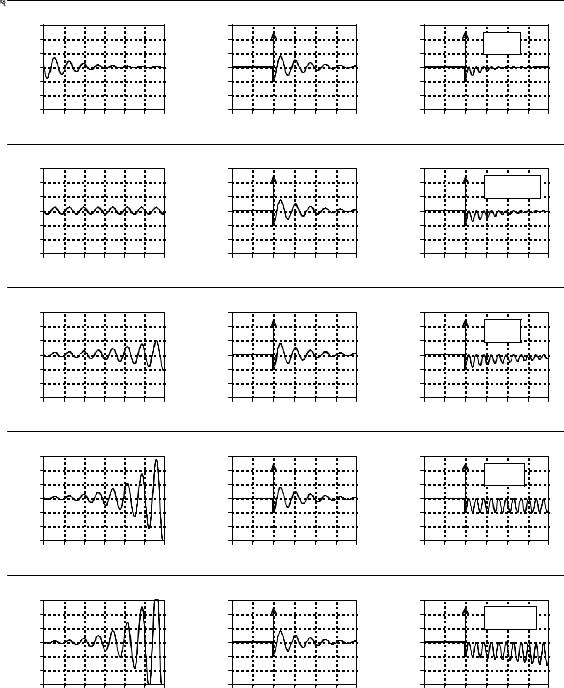
592 |
The Scientist and Engineer's Guide to Digital Signal Processing |
cannot cancel a decreasing impulse response. This means that a stable system will not have any poles with F > 0 . In other words, all of the poles in a stable system are confined to the left half of the s-plane. In fact, poles in the right half of the s-place show that the system is unstable (i.e., an impulse response that increases with time).
Figure (b) shows one of the special cases we have been looking for. When this waveform is multiplied by the impulse response, the resulting integral has a value of zero. This occurs because the area above the x-axis (from the delta function) is exactly equal to the area below (from the rectified sinusoid). The values for F and T that produce this type of cancellation are called a zero of the system. As shown in the s-plane diagram of Fig. 32-4, zeros are indicated by small circles (•).
Figure (c) shows the next probe we can try. Here we are using a sinusoid that exponentially increases with time, but at a rate slower than the impulse response is decreasing with time. This results in the product of the two waveforms also decreasing as time advances. As in (a), this makes the integral of the product some uninteresting real number. The important point being that no type of exact cancellation occurs.
Jumping out of order, look at (e), a probing waveform that increases at a faster rate than the impulse response decays. When multiplied, the resulting signal increases in amplitude as time advances. This means that the area under the curve becomes larger with increasing time, and the total area from t ' & 4 to % 4 is not defined. In mathematical jargon, the integral does not converge. In other words, not all areas of the s-plane have a defined value. The portion of the s-plane where the integral is defined is called the region-of- convergence. In some mathematical techniques it is important to know what portions of the s-plane are within the region-of-convergence. However, this information is not needed for the applications in this book. Only the exact cancellations are of interest for this discussion.
In (d), the probing waveform increases at exactly the same rate that the impulse response decreases. This makes the product of the two waveforms have a constant amplitude. In other words, this is the dividing line between (c) and (e), resulting in a total area that is just barely undefined (if the mathematicians will forgive this loose description). In more exact terms, this point is on the borderline of the region of convergence. As mentioned, values for F and T that produce this type of exact cancellation are called poles of the system. Poles are indicated in the s-plane by crosses (×).
Analysis of Electric Circuits
We have introduced the Laplace transform in graphical terms, describing what the waveforms look like and how they are manipulated. This is the most intuitive way of understanding the approach, but is very different from how it is actually used. The Laplace transform is inherently a mathematical technique; it is used by writing and manipulating equations. The problem is, it is easy to

Chapter 32The Laplace Transform |
593 |
become lost in the abstract nature of the complex algebra and loose all connection to the real world. Your task is to merge the two views together. The Laplace transform is the primary method for analyzing electric circuits. Keep in mind that any system governed by differential equations can be handled the same way; electric circuits are just an example we are using.
The brute force approach is to solve the differential equations controlling the system, providing the system's impulse response. The impulse response can then be converted into the s-domain via Eq. 32-1. Fortunately, there is a better way: transform each of the individual components into the s-domain, and then account for how they interact. This is very similar to the phasor transform presented in Chapter 30, where resistors, inductors and capacitors are represented by R, jTL , and 1 / jTC , respectively. In the Laplace transform, resistors, inductors and capacitors become the complex variables: R, s L , and 1/sC . Notice that the phasor transform is a subset of the Laplace transform. That is, when F is set to zero in s ' F% jT, R becomes R, s L becomes jTL , and 1/sC becomes 1 / jTC .
Just as in Chapter 30, we will treat each of the three components as an individual system, with the current waveform being the input signal, and the voltage waveform being the output signal. When we say that resistors, inductors and capacitors become R, s L , and 1/sC in the s-domain, this refers to the output divided by the input. In other words, the Laplace transform of the voltage waveform divided by the Laplace transform of the current waveform is equal to these expressions.
As an example of this, imagine we force the current through an inductor to be a unity amplitude cosine wave with a frequency given by T0. The resulting voltage waveform across the inductor can be found by solving the differential equation that governs its operation:
v (t ) ' L |
d |
i (t ) ' |
L |
d |
cos (T t ) ' |
T L sin(T t ) |
|
|
|
||||||
|
dt |
|
dt |
0 |
0 |
0 |
|
|
|
|
|
|
|||
If we start the current waveform at t ' 0 , the voltage waveform will also start
at this same time (i.e., i (t ) ' 0 and v (t ) ' 0 for |
t < 0 ). |
These voltage and |
||||||||
current waveforms are converted into the s-domain by Eq. 32-1: |
||||||||||
|
|
4 |
|
|
|
|
|
T0 |
||
I (s) |
' |
m |
cos (T t ) e &st d t |
' |
|
|||||
|
|
|
|
|||||||
|
|
0 |
|
|
|
T2 % s 2 |
||||
|
|
|
|
|
|
|||||
|
|
0 |
|
|
|
0 |
|
|
||
|
|
4 |
|
|
|
|
|
T0 L s |
|
|
V (s) ' |
m T0 L sin(T0 t ) e |
&s t |
d t |
' |
|
|||||
|
|
T2 % s 2 |
||||||||
|
|
0 |
|
|
|
|
|
0 |
|
|

594 |
The Scientist and Engineer's Guide to Digital Signal Processing |
To complete this example, we will divide the s-domain voltage by the s-domain current, just as if we were using Ohm's law ( R ' V / I ):
|
|
|
T0 L s |
|
|
V (s) |
|
|
T2 % s 2 |
|
|
' |
0 |
|
' sL |
||
I (s) |
|
T0 |
|
||
|
|
|
|||
|
|
|
T2 % s 2 |
|
|
|
|
0 |
|
|
|
We find that the s-domain representation of the voltage across the inductor, divided by the s-domain representation of the current through the inductor, is equal to sL. This is always the case, regardless of the current waveform we start with. In a similar way, the ratio of s-domain voltage to s-domain current is always equal to R for resistors, and 1/sC for capacitors.
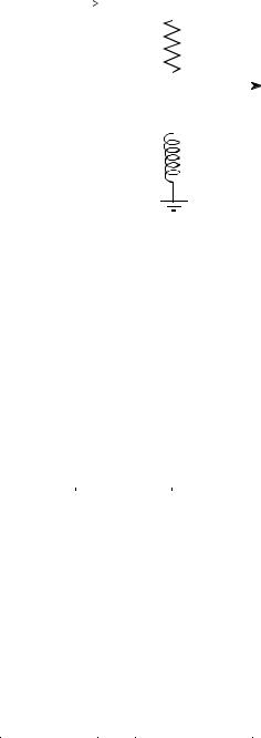
Figure 32-6 shows an example circuit we will analyze with the Laplace transform, the RLC notch filter discussed in Chapter 30. Since this analysis is the same for all electric circuits, we will outline it in steps.
Step 1. Transform each of the components into the s-domain. In other words, replace the value of each resistor with R, each inductor with sL , and each capacitor with 1/sC . This is shown in Fig. 32-6.
Step 2: Find H (s), the output divided by the input. As described in Chapter 30, this is done by treating each of the components as if they obey Ohm's law, with the "resistances" given by: R, s L , and 1/sC . This allows us to use the standard equations for resistors in series, resistors in parallel, voltage dividers, etc. Treating the RLC circuit in this example as a voltage divider (just as in Chapter 30), H (s) is found:
H (s) ' |
Vout (s) |
' |
sL % 1/sC |
' |
sL % 1/sC |
|
|
s |
|
' |
L s 2 % 1/C |
Vin (s) |
R % sL % 1/sC |
R % sL % 1/sC |
|
|
s |
|
L s 2 % Rs % 1/C |
||||
|
|
|
|
|
|
|
|||||
|
|
|
|
|
|
As you recall from Fourier analysis, the frequency spectrum of the output signal divided by the frequency spectrum of the input signal is equal to the system's frequency response, given the symbol, H (T) . The above equation is an extension of this into the s-domain. The signal, H (s ) , is called the system's transfer function, and is equal to the s-domain representation of the output signal divided by the s-domain representation of the input signal. Further, H (s) is equal to the Laplace transform of the impulse response, just the same as H (T) is equal to the Fourier transform of the impulse response.
Chapter 32The Laplace Transform |
595 |
|||||
|
Vin |
|
|
|
||
|
|
|
|
|
|
|
|
|
|
|
|
|
|
FIGURE 32-6 |
|
R |
|
|
|
|
|
|
|
|
Vout |
||
Notch filter analysis in the s-domain. The |
|
|
|
|
||
|
|
|
||||
first step in this procedure is to replace the |
|
|
|
|
|
|
|
|
|
|
|
|
|
resistor, inductor & capacitor values with |
|
1/sC |
|
|
|
|
their s-domain equivalents. |
|
|
|
|
|
|
|
|
|
|
|
|
|
|
|
|
|
|
|
|
sL
So far, this is identical to the techniques of the last chapter, except for using s instead of jT. The difference between the two methods is what happens from this point on. This is as far as we can go with jT. We might graph the frequency response, or examining it in some other way; however, this is a mathematical dead end. In comparison, the interesting aspects of the Laplace transform have just begun. Finding H (s) is the key to Laplace analysis; however, it must be expressed in a particular form to be useful. This requires the algebraic manipulation of the next two steps.
Step 3: Arrange H (s) to be one polynomial over another. This makes the transfer function written as:
EQUATION 32-2 |
H (s) ' |
a s 2 % b s % c |
|
Transfer function in polynomial form. |
a s 2 % b s % c |
||
|
|||
|
|
It is always possible to express the transfer function in this form if the system is controlled by differential equations. For example, the rectangular pulse shown in Fig. 32-3 is not the solution to a differential equation and its Laplace transform cannot be written in this way. In comparison, any electric circuit composed of resistors, capacitors, and inductors can be written in this form. For the RLC notch filter used in this example, the algebra shown in step 2 has already placed the transfer function in the correct form, that is:
H (s) ' |
a s 2 % b s % c |
' |
L s 2 % 1/C |
|
a s 2 % bs % c |
L s 2 % R s % 1/C |
|||
|
|
where: a ' L , b ' 0, c ' 1/C ; and a ' L , b ' R, c ' 1/C
Step 4: Factor the numerator and denominator polynomials. That is, break the numerator and denominator polynomials into components that each contain