

Digital Signal Processing. The Scientist and Engineers Guide. Steven W. Smith
.pdf
|
Chapter 2- Statistics, Probability and Noise |
17 |
|
100 'MEAN AND STANDARD DEVIATION USING RUNNING STATISTICS |
|
||
110 ' |
|
|
|
120 |
DIM X[511] |
'The signal is held in X[0] to X[511] |
|
130 ' |
|
|
|
140 |
GOSUB XXXX |
'Mythical subroutine that loads the signal into X[ ] |
|
150 ' |
|
|
|
160 N% = 0 |
'Zero the three running parameters |
|
|
170 SUM = 0 |
|
|
|
180 SUMSQUARES = 0 |
|
|
|
190 ' |
|
|
|
200 |
FOR I% = 0 TO 511 |
'Loop through each sample in the signal |
|
210 |
' |
|
|
220 |
N% = N%+1 |
'Update the three parameters |
|
230 |
SUM = SUM + X[I%] |
|
|
240 |
SUMSQUARES = SUMSQUARES + X[I%]^2 |
|
|
250 |
' |
|
|
260 |
MEAN = SUM/N% |
'Calculate mean and standard deviation via Eq. 2-3 |
|
270 |
IF N% = 1 THEN SD = 0: GOTO 300 |
|
|
280 |
SD = SQR( (SUMSQUARES - SUM^2/N%) / (N%-1) ) |
|
|
290 |
' |
|
|
300 |
PRINT MEAN SD |
'Print the running mean and standard deviation |
|
310 |
' |
|
|
320 NEXT I%
330 '
340 END
TABLE 2-2
Before ending this discussion on the mean and standard deviation, two other terms need to be mentioned. In some situations, the mean describes what is being measured, while the standard deviation represents noise and other interference. In these cases, the standard deviation is not important in itself, but only in comparison to the mean. This gives rise to the term: signal-to-noise ratio (SNR), which is equal to the mean divided by the standard deviation. Another term is also used, the coefficient of variation (CV). This is defined as the standard deviation divided by the mean, multiplied by 100 percent. For example, a signal (or other group of measure values) with a CV of 2%, has an SNR of 50. Better data means a higher value for the SNR and a lower value for the CV.
Signal vs. Underlying Process
Statistics is the science of interpreting numerical data, such as acquired signals. In comparison, probability is used in DSP to understand the processes that generate signals. Although they are closely related, the distinction between the acquired signal and the underlying process is key to many DSP techniques.
For example, imagine creating a 1000 point signal by flipping a coin 1000 times. If the coin flip is heads, the corresponding sample is made a value of one. On tails, the sample is set to zero. The process that created this signal has a mean of exactly 0.5, determined by the relative probability of each possible outcome: 50% heads, 50% tails. However, it is unlikely that the actual 1000 point signal will have a mean of exactly 0.5. Random chance

18 |
The Scientist and Engineer's Guide to Digital Signal Processing |
will make the number of ones and zeros slightly different each time the signal is generated. The probabilities of the underlying process are constant, but the statistics of the acquired signal change each time the experiment is repeated. This random irregularity found in actual data is called by such names as: statistical variation, statistical fluctuation, and statistical noise.
This presents a bit of a dilemma. When you see the terms: mean and standard deviation, how do you know if the author is referring to the statistics of an actual signal, or the probabilities of the underlying process that created the signal? Unfortunately, the only way you can tell is by the context. This is not so for all terms used in statistics and probability. For example, the histogram and probability mass function (discussed in the next section) are matching concepts that are given separate names.
Now, back to Eq. 2-2, calculation of the standard deviation. As previously mentioned, this equation divides by N-1 in calculating the average of the squared deviations, rather than simply by N. To understand why this is so, imagine that you want to find the mean and standard deviation of some process that generates signals. Toward this end, you acquire a signal of N samples from the process, and calculate the mean of the signal via Eq. 2.1. You can then use this as an estimate of the mean of the underlying process; however, you know there will be an error due to statistical noise. In particular, for random signals, the typical error between the mean of the N points, and the mean of the underlying process, is given by:
EQUATION 2-4
Typical error in calculating the mean of an underlying process by using a finite number of samples, N. The parameter, σ , is the standard deviation.
F
Typical error '
N 1/2
If N is small, the statistical noise in the calculated mean will be very large. In other words, you do not have access to enough data to properly characterize the process. The larger the value of N, the smaller the expected error will become. A milestone in probability theory, the Strong Law of Large Numbers, guarantees that the error becomes zero as N approaches infinity.
In the next step, we would like to calculate the standard deviation of the acquired signal, and use it as an estimate of the standard deviation of the underlying process. Herein lies the problem. Before you can calculate the standard deviation using Eq. 2-2, you need to already know the mean, µ. However, you don't know the mean of the underlying process, only the mean of the N point signal, which contains an error due to statistical noise. This error tends to reduce the calculated value of the standard deviation. To compensate for this, N is replaced by N-1. If N is large, the difference doesn't matter. If N is small, this replacement provides a more accurate
Chapter 2- Statistics, Probability and Noise |
19 |
|
8 |
|
|
|
|
|
|
|
|
|
|
a. Changing mean and standard deviation |
|
|
|||||
|
6 |
|
|
|
|
|
|
|
|
Amplitude |
4 |
|
|
|
|
|
|
|
|
2 |
|
|
|
|
|
|
|
|
|
0 |
|
|
|
|
|
|
|
|
|
|
|
|
|
|
|
|
|
|
|
|
-2 |
|
|
|
|
|
|
|
|
|
-4 |
|
|
|
|
|
|
|
|
|
0 |
64 |
128 |
192 |
256 |
320 |
384 |
448 |
5121 |
Sample number
|
8 |
|
|
|
|
|
|
|
|
|
|
b. Changing mean, constant standard deviation |
|
||||||
|
6 |
|
|
|
|
|
|
|
|
Amplitude |
4 |
|
|
|
|
|
|
|
|
2 |
|
|
|
|
|
|
|
|
|
0 |
|
|
|
|
|
|
|
|
|
|
|
|
|
|
|
|
|
|
|
|
-2 |
|
|
|
|
|
|
|
|
|
-4 |
|
|
|
|
|
|
|
|
|
0 |
64 |
128 |
192 |
256 |
320 |
384 |
448 |
5121 |
Sample number
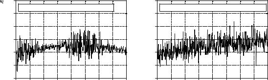
FIGURE 2-3
Examples of signals generated from nonstationary processes. In (a), both the mean and standard deviation change. In (b), the standard deviation remains a constant value of one, while the mean changes from a value of zero to two. It is a common analysis technique to break these signals into short segments, and calculate the statistics of each segment individually.
estimate of the standard deviation of the underlying process. In other words, Eq. 2-2 is an estimate of the standard deviation of the underlying process. If we divided by N in the equation, it would provide the standard deviation of the acquired signal.
As an illustration of these ideas, look at the signals in Fig. 2-3, and ask: are the variations in these signals a result of statistical noise, or is the underlying process changing? It probably isn't hard to convince yourself that these changes are too large for random chance, and must be related to the underlying process. Processes that change their characteristics in this manner are called nonstationary. In comparison, the signals previously presented in Fig. 2-1 were generated from a stationary process, and the variations result completely from statistical noise. Figure 2-3b illustrates a common problem with nonstationary signals: the slowly changing mean interferes with the calculation of the standard deviation. In this example, the standard deviation of the signal, over a short interval, is one. However, the standard deviation of the entire signal is 1.16. This error can be nearly eliminated by breaking the signal into short sections, and calculating the statistics for each section individually. If needed, the standard deviations for each of the sections can be averaged to produce a single value.
The Histogram, Pmf and Pdf
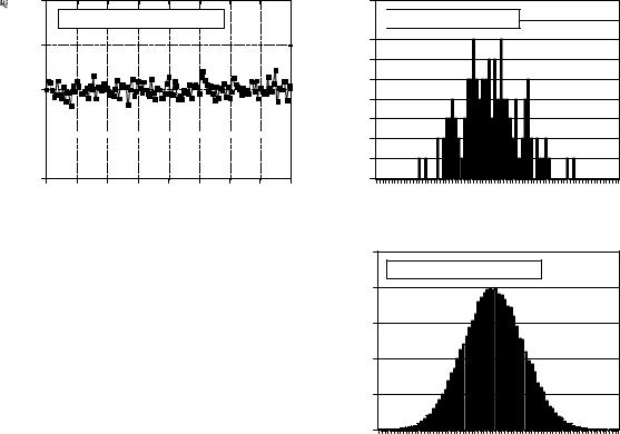
Suppose we attach an 8 bit analog-to-digital converter to a computer, and acquire 256,000 samples of some signal. As an example, Fig. 2-4a shows 128 samples that might be a part of this data set. The value of each sample will be one of 256 possibilities, 0 through 255. The histogram displays the number of samples there are in the signal that have each of these possible values. Figure (b) shows the histogram for the 128 samples in (a). For
20 |
The Scientist and Engineer's Guide to Digital Signal Processing |
|
255 |
|
|
a. 128 samples of 8 bit signal |
|
Amplitude |
192 |
|
128 |
||
|
64 


0
0 |
16 |
32 |
48 |
64 |
80 |
96 |
112 |
1287 |
Sample number
 Number of occurences
9
8  b. 128 point histogram
7
6
5
4
3
2
1
0
90 |
100 |
110 |
120 |
130 |
140 |
150 |
160 |
170 |
Value of sample
FIGURE 2-4
Examples of histograms. Figure (a) shows 128 samples from a very long signal, with each sample being an integer between 0 and 255. Figures (b) and (c) show histograms using 128 and 256,000 samples from the signal, respectively. As shown, the histogram is smoother when more samples are used.
10000
|
c. 256,000 point histogram |
|
occurencesof |
8000 |
|
6000 |
||
Number |
||
4000 |
||
|
||
|
2000 |
0 |
|
|
|
|
|
|
|
|
90 |
100 |
110 |
120 |
130 |
140 |
150 |
160 |
170 |
Value of sample
example, there are 2 samples that have a value of 110, 7 samples that have a value of 131, 0 samples that have a value of 170, etc. We will represent the histogram by Hi, where i is an index that runs from 0 to M-1, and M is the number of possible values that each sample can take on. For instance, H50 is the number of samples that have a value of 50. Figure (c) shows the histogram of the signal using the full data set, all 256k points. As can be seen, the larger number of samples results in a much smoother appearance. Just as with the mean, the statistical noise (roughness) of the histogram is inversely proportional to the square root of the number of samples used.
From the way it is defined, the sum of all of the values in the histogram must be equal to the number of points in the signal:
EQUATION 2-5
The sum of all of the values in the histogram is equal to the number of points in the signal. In this equation, Hi is the histogram, N is the number of points in the signal, and M is the number of points in the histogram.
M&1
N ' j Hi
i ' 0
The histogram can be used to efficiently calculate the mean and standard deviation of very large data sets. This is especially important for images, which can contain millions of samples. The histogram groups samples

Chapter 2- Statistics, Probability and Noise |
21 |
together that have the same value. This allows the statistics to be calculated by working with a few groups, rather than a large number of individual samples. Using this approach, the mean and standard deviation are calculated from the histogram by the equations:
EQUATION 2-6
Calculation of the mean from the histogram. This can be viewed as combining all samples having the same value into groups, and then using Eq. 2-1 on each group.
EQUATION 2-7
Calculation of the standard deviation from the histogram. This is the same concept as Eq. 2-2, except that all samples having the same value are operated on at once.
|
|
1 |
M&1 |
||
µ |
' |
j i Hi |
|||
|
|
||||
N |
|||||
|
|
i ' 0 |
|||
|
1 |
|
M &1 |
||
F2 ' |
|
j (i & µ )2 Hi |
|||
|
|
||||
|
|
||||
|
N & 1 i '0 |
||||
Table 2-3 contains a program for calculating the histogram, mean, and standard deviation using these equations. Calculation of the histogram is very fast, since it only requires indexing and incrementing. In comparison,
100 |
'CALCULATION OF THE HISTOGRAM, MEAN, AND STANDARD DEVIATION |
|
110 |
' |
|
120 |
DIM X%[25000] |
'X%[0] to X%[25000] holds the signal being processed |
130 |
DIM H%[255] |
'H%[0] to H%[255] holds the histogram |
140 N% = 25001 |
'Set the number of points in the signal |
|
150 |
' |
|
160 |
FOR I% = 0 TO 255 |
'Zero the histogram, so it can be used as an accumulator |
170 |
H%[I%] = 0 |
|
180 NEXT I% |
|
|
190 |
' |
|
200 |
GOSUB XXXX |
'Mythical subroutine that loads the signal into X%[ ] |
210 |
' |
|
220 |
FOR I% = 0 TO 25000 'Calculate the histogram for 25001 points |
|
230 |
H%[ X%[I%] ] = H%[ X%[I%] ] + 1 |
|
240 NEXT I% |
|
|
250 |
' |
|
260 |
MEAN = 0 |
'Calculate the mean via Eq. 2-6 |
270 FOR I% = 0 TO 255 |
|
|
280 |
MEAN = MEAN + I% * H%[I%] |
|
290 NEXT I% |
|
|
300 MEAN = MEAN / N% |
|
|
310 |
' |
|
320 |
VARIANCE = 0 |
'Calculate the standard deviation via Eq. 2-7 |
330 FOR I% = 0 TO 255 |
|
|
340 |
VARIANCE = VARIANCE + H%[I%] * (I%-MEAN)^2 |
|
350 NEXT I% |
|
|
360 VARIANCE = VARIANCE / (N%-1) |
||
370 SD = SQR(VARIANCE) |
|
|
380 |
' |
|
390 |
PRINT MEAN SD |
'Print the calculated mean and standard deviation. |
400 |
' |
|
410 END |
TABLE 2-3 |
|
|
|
|
22 |
The Scientist and Engineer's Guide to Digital Signal Processing |
calculating the mean and standard deviation requires the time consuming operations of addition and multiplication. The strategy of this algorithm is to use these slow operations only on the few numbers in the histogram, not the many samples in the signal. This makes the algorithm much faster than the previously described methods. Think a factor of ten for very long signals with the calculations being performed on a general purpose computer.
The notion that the acquired signal is a noisy version of the underlying process is very important; so important that some of the concepts are given different names. The histogram is what is formed from an acquired signal. The corresponding curve for the underlying process is called the probability mass function (pmf). A histogram is always calculated using a finite number of samples, while the pmf is what would be obtained with an infinite number of samples. The pmf can be estimated (inferred) from the histogram, or it may be deduced by some mathematical technique, such as in the coin flipping example.
Figure 2-5 shows an example pmf, and one of the possible histograms that could be associated with it. The key to understanding these concepts rests in the units of the vertical axis. As previously described, the vertical axis of the histogram is the number of times that a particular value occurs in the signal. The vertical axis of the pmf contains similar information, except expressed on a fractional basis. In other words, each value in the histogram is divided by the total number of samples to approximate the pmf. This means that each value in the pmf must be between zero and one, and that the sum of all of the values in the pmf will be equal to one.
The pmf is important because it describes the probability that a certain value will be generated. For example, imagine a signal with the pmf of Fig. 2-5b, such as previously shown in Fig. 2-4a. What is the probability that a sample taken from this signal will have a value of 120? Figure 2-5b provides the answer, 0.03, or about 1 chance in 34. What is the probability that a randomly chosen sample will have a value greater than 150? Adding up the values in the pmf for: 151, 152, 153,@@@, 255, provides the answer, 0.0122, or about 1 chance in 82. Thus, the signal would be expected to have a value exceeding 150 on an average of every 82 points. What is the probability that any one sample will be between 0 and 255? Summing all of the values in the pmf produces the probability of 1.00, that is, a certainty that this will occur.
The histogram and pmf can only be used with discrete data, such as a digitized signal residing in a computer. A similar concept applies to continuous signals, such as voltages appearing in analog electronics. The probability density function (pdf), also called the probability distribution function, is to continuous signals what the probability mass function is to discrete signals. For example, imagine an analog signal passing through an analog-to-digital converter, resulting in the digitized signal of Fig. 2-4a. For simplicity, we will assume that voltages between 0 and 255 millivolts become digitized into digital numbers between 0 and 255. The pmf of this digital
Chapter 2- Statistics, Probability and Noise |
23 |
|
10000 |
|
|
|
|
|
|
|
|
|
0.060 |
|
|
|
|
|
|
|
|
|
|
a. Histogram |
|
|
|
|
|
|
|
|
b. Probability Mass Function (pmf) |
|
|
||||||
Number of occurences |
8000 |
|
|
|
|
|
|
|
|
Probability of occurence |
0.050 |
|
|
|
|
|
|
|
|
|
|
|
|
|
|
|
|
|
|
|
|
|
|
|
|
|
|||
|
|
|
|
|
|
|
|
|
0.040 |
|
|
|
|
|
|
|
|
||
6000 |
|
|
|
|
|
|
|
|
|
|
|
|
|
|
|
|
|
||
|
|
|
|
|
|
|
|
|
0.030 |
|
|
|
|
|
|
|
|
||
4000 |
|
|
|
|
|
|
|
|
|
|
|
|
|
|
|
|
|
||
|
|
|
|
|
|
|
|
|
0.020 |
|
|
|
|
|
|
|
|
||
2000 |
|
|
|
|
|
|
|
|
0.010 |
|
|
|
|
|
|
|
|
||
|
|
|
|
|
|
|
|
|
|
|
|
|
|
|
|
|
|
||
|
|
|
|
|
|
|
|
|
|
|
|
|
|
|
|
|
|
|
|
|
0 |
|
|
|
|
|
|
|
|
|
0.000 |
|
|
|
|
|
|
|
|
|
90 |
100 |
110 |
120 |
130 |
140 |
150 |
160 |
170 |
|
90 |
100 |
110 |
120 |
130 |
140 |
150 |
160 |
170 |
Value of sample |
Value of sample |
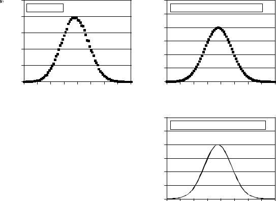
FIGURE 2-5
The relationship between (a) the histogram, (b) the probability mass function (pmf), and (c) the probability density function (pdf). The histogram is calculated from a finite number of samples. The pmf describes the probabilities of the underlying process. The pdf is similar to the pmf, but is used with continuous rather than discrete signals. Even though the vertical axis of (b) and (c) have the same values (0 to 0.06), this is only a coincidence of this example. The amplitude of these three curves is determined by:
(a) the sum of the values in the histogram being equal to the number of samples in the signal; (b) the sum of the values in the pmf being equal to one, and (c) the area under the pdf curve being equal to one.
 Probability density
0.060
c. Probability Density Function (pdf)
0.050
0.040
0.030
0.020
0.010
0.000
90 |
100 |
110 |
120 |
130 |
140 |
150 |
160 |
170 |
Signal level (millivolts)
signal is shown by the markers in Fig. 2-5b. Similarly, the pdf of the analog signal is shown by the continuous line in (c), indicating the signal can take on a continuous range of values, such as the voltage in an electronic circuit.
The vertical axis of the pdf is in units of probability density, rather than just probability. For example, a pdf of 0.03 at 120.5 does not mean that the a voltage of 120.5 millivolts will occur 3% of the time. In fact, the probability of the continuous signal being exactly 120.5 millivolts is infinitesimally small. This is because there are an infinite number of possible values that the signal needs to divide its time between: 120.49997, 120.49998, 120.49999, etc. The chance that the signal happens to be exactly 120.50000þ is very remote indeed!
To calculate a probability, the probability density is multiplied by a range of values. For example, the probability that the signal, at any given instant, will be between the values of 120 and 121 is: (121&120) × 0.03 ' 0.03. The p r o b a b i l i t y t h a t t h e s i g n a l w i l l b e b e t w e e n 1 2 0 . 4 a n d 1 2 0 . 5 i s : (120.5&120.4) × 0.03 ' 0.003 , etc. If the pdf is not constant over the range of interest, the multiplication becomes the integral of the pdf over that range. In other words, the area under the pdf bounded by the specified values. Since the value of the signal must always be something, the total area under the pdf
24 |
The Scientist and Engineer's Guide to Digital Signal Processing |
curve, the integral from &4 to %4, will always be equal to one. This is analogous to the sum of all of the pmf values being equal to one, and the sum of all of the histogram values being equal to N.
The histogram, pmf, and pdf are very similar concepts. Mathematicians always keep them straight, but you will frequently find them used interchangeably (and therefore, incorrectly) by many scientists and
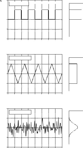
FIGURE 2-6
Three common waveforms and their probability density functions. As in these examples, the pdf graph is often rotated one-quarter turn and placed at the side of the signal it describes. The pdf of a square wave, shown in (a), consists of two infinitesimally narrow spikes, corresponding to the signal only having two possible values. The pdf of the triangle wave, (b), has a constant value over a range, and is often called a uniform distribution. The pdf of random noise, as in (c), is the most interesting of all, a bell shaped curve known as a
Gaussian.
2


 pdf a. Square wave


1 


Amplitude |
0 |
|
|
|
|
|
|
|
|
|
|
|
|
|
|
|
|
|
|
|
-1 |
|
|
|
|
|
|
|
|
|
-2 |
|
|
|
|
|
|
|
|
|
0 |
16 |
32 |
48 |
64 |
80 |
96 |
112 |
1278 |
Time (or other variable)
|
2 |
|
|
|
|
|
|
|
|
|
|
b. Triangle wave |
|
|
|
|
|||
|
|
|
|
|
|
|
|||
Amplitude |
1 |
|
|
|
|
|
|
|
|
0 |
|
|
|
|
|
|
|
|
|
|
|
|
|
|
|
|
|
|
|
|
-1 |
|
|
|
|
|
|
|
|
|
-2 |
|
|
|
|
|
|
|
|
|
0 |
16 |
32 |
48 |
64 |
80 |
96 |
112 |
1278 |
|
|
|
Time (or other variable) |
|
|
|
|||
|
2 |
c. Random noise |
|
|
|
|
|||
|
|
|
|
|
|
|
|||
Amplitude |
1 |
|
|
|
|
|
|
|
|
0 |
|
|
|
|
|
|
|
|
|
|
|
|
|
|
|
|
|
|
|
|
-1 |
|
|
|
|
|
|
|
|
|
-2 |
|
|
|
|
|
|
|
|
|
0 |
16 |
32 |
48 |
64 |
80 |
96 |
112 |
1287 |
Time (or other variable)
Chapter 2- Statistics, Probability and Noise |
25 |
engineers. Figure 2-6 shows three continuous waveforms and their pdfs. If these were discrete signals, signified by changing the horizontal axis labeling to "sample number," pmfs would be used.
A problem occurs in calculating the histogram when the number of levels each sample can take on is much larger than the number of samples in the signal. This is always true for signals represented in floating point notation, where each sample is stored as a fractional value. For example, integer representation might require the sample value to be 3 or 4, while floating point allows millions of possible fractional values between 3 and 4. The previously described approach for calculating the histogram involves counting the number of samples that have each of the possible quantization levels. This is not possible with floating point data because there are billions of possible levels that would have to be taken into account. Even worse, nearly all of these possible levels would have no samples that correspond to them. For example, imagine a 10,000 sample signal, with each sample having one billion possible values. The conventional histogram would consist of one billion data points, with all but about 10,000 of them having a value of zero.
The solution to these problems is a technique called binning. This is done by arbitrarily selecting the length of the histogram to be some convenient number, such as 1000 points, often called bins. The value of each bin represents the total number of samples in the signal that have a value within a certain range. For example, imagine a floating point signal that contains values between 0.0 and 10.0, and a histogram with 1000 bins. Bin 0 in the histogram is the number of samples in the signal with a value between 0 and 0.01, bin 1 is the number of samples with a value between 0.01 and 0.02, and so forth, up to bin 999 containing the number of samples with a value between 9.99 and 10.0. Table 2-4 presents a program for calculating a binned histogram in this manner.
100 'CALCULATION OF BINNED HISTOGRAM
110 '
120 |
DIM X[25000] |
'X[0] to X[25000] holds the floating point signal, |
130 ' |
'with each sample having a value between 0.0 and 10.0. |
|
140 |
DIM H%[999] |
'H%[0] to H%[999] holds the binned histogram |
150 ' |
|
|
160 |
FOR I% = 0 TO 999 |
'Zero the binned histogram for use as an accumulator |
170 |
H%[I%] = 0 |
|
180 NEXT I% |
|
|
190 ' |
|
|
200 |
GOSUB XXXX |
'Mythical subroutine that loads the signal into X%[ ] |
210 ' |
|
|
220 |
FOR I% = 0 TO 25000 ' |
'Calculate the binned histogram for 25001 points |
230 |
BINNUM% = INT( X[I%] * 100 ) |
|
240 |
H%[ BINNUM%] = H%[ BINNUM%] + 1 |
|
250 NEXT I%
260 '
270 END
TABLE 2-4
26 |
|
|
The Scientist and Engineer's Guide to Digital Signal Processing |
|||||
4 |
|
|
|
|
0.8 |
|
|
|
|
|
|
|
|
|
|
||
|
|
a. |
Example signal |
|
|
|
b. Histogram of 601 bins |
|
|
|
|
|
|
|
|
|
|
Amplitude |
1 |
ofNumberoccurences |
0.2 |
|
3 |
|
0.6 |
|
2 |
|
0.4 |
0 |
|
|
|
|
|
|
0 |
|
|
|
|
0 |
50 |
100 |
150 |
200 |
250 |
300 |
0 |
150 |
300 |
450 |
600 |
|
|
Sample number |
|
|
|
Bin number in histogram |
|
||||
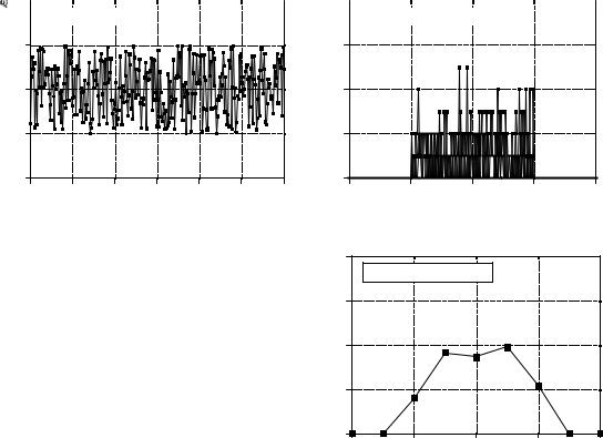
FIGURE 2-7
Example of binned histograms. As shown in (a), the signal used in this example is 300 samples long, with each sample a floating point number uniformly distributed between 1 and 3. Figures (b) and (c) show binned histograms of this signal, using 601 and 9 bins, respectively. As shown, a large number of bins results in poor resolution along the vertical axis, while a small number of bins provides poor resolution along the horizontal axis. Using more samples makes the resolution better in both directions.
|
160 |
|
|
|
|
occurences |
|
c. Histogram of 9 bins |
|
|
|
120 |
|
|
|
|
|
|
|
|
|
|
|
Number of |
80 |
|
|
|
|
40 |
|
|
|
|
|
|
0 |
|
|
|
|
|
0 |
2 |
4 |
6 |
8 |
Bin number in histogram
How many bins should be used? This is a compromise between two problems. As shown in Fig. 2-7, too many bins makes it difficult to estimate the amplitude of the underlying pmf. This is because only a few samples fall into each bin, making the statistical noise very high. At the other extreme, too few of bins makes it difficult to estimate the underlying pmf in the horizontal direction. In other words, the number of bins controls a tradeoff between resolution along the y-axis, and resolution along the x-axis.
The Normal Distribution
Signals formed from random processes usually have a bell shaped pdf. This is called a normal distribution, a Gauss distribution, or a Gaussian, after the great German mathematician, Karl Friedrich Gauss (1777-1855). The reason why this curve occurs so frequently in nature will be discussed shortly in conjunction with digital noise generation. The basic shape of the curve is generated from a negative squared exponent:
y (x ) ' e & x 2