456 |
PART EIGHT SHORT-RUN ECONOMIC FLUCTUATIONS |
increasing the money supply and lowering interest rates. The federal funds rate fell from 7.7 percent at the beginning of October to 6.6 percent at the end of the month. In part because of the Fed’s quick action, the economy avoided a recession.
While the Fed keeps an eye on the stock market, stock-market participants also keep an eye on the Fed. Because the Fed can influence interest rates and economic activity, it can alter the value of stocks. For example, when the Fed raises interest rates by reducing the money supply, it makes owning stocks less attractive for two reasons. First, a higher interest rate means that bonds, the alternative to stocks, are earning a higher return. Second, the Fed’s tightening of monetary policy risks pushing the economy into a recession, which reduces profits. As a result, stock prices often fall when the Fed raises interest rates.
QUICK QUIZ: Use the theory of liquidity preference to explain how a de crease in the money supply affects the equilibrium interest rate. How does this change in monetary policy affect the aggregate-demand curve?
HOW FISCAL POLICY
INFLUENCES AGGREGATE DEMAND
The government can influence the behavior of the economy not only with monetary policy but also with fiscal policy. Fiscal policy refers to the government’s choices regarding the overall level of government purchases or taxes. Earlier in the book we examined how fiscal policy influences saving, investment, and growth in the long run. In the short run, however, the primary effect of fiscal policy is on the aggregate demand for goods and services.
CHANGES IN GOVERNMENT PURCHASES
When policymakers change the money supply or the level of taxes, they shift the aggregate-demand curve by influencing the spending decisions of firms or households. By contrast, when the government alters its own purchases of goods and services, it shifts the aggregate-demand curve directly.
Suppose, for instance, that the U.S. Department of Defense places a $20 billion order for new fighter planes with Boeing, the large aircraft manufacturer. This order raises the demand for the output produced by Boeing, which induces the company to hire more workers and increase production. Because Boeing is part of the economy, the increase in the demand for Boeing planes means an increase in the total quantity of goods and services demanded at each price level. As a result, the aggregate-demand curve shifts to the right.
By how much does this $20 billion order from the government shift the aggregate-demand curve? At first, one might guess that the aggregate-demand curve shifts to the right by exactly $20 billion. It turns out, however, that this is not
458 |
PART EIGHT SHORT-RUN ECONOMIC FLUCTUATIONS |
Figur e 20-4
THE MULTIPLIER EFFECT. An
increase in government purchases of $20 billion can shift the aggregate-demand curve to the right by more than $20 billion. This multiplier effect arises because increases in aggregate income
stimulate additional spending by consumers.
Price
Level
2. . . . but the multiplier effect can amplify the shift in aggregate demand.
$20 billion
|
|
|
AD3 |
|
|
|
AD2 |
|
|
Aggregate demand, AD1 |
|
|
|
|
0 |
|
|
Quantity of |
|
|
1. An increase in government purchases |
Output |
|
|
of $20 billion initially increases aggregate |
|
|
|
demand by $20 billion . . . |
|
|
|
|
|
To gauge the impact on aggregate demand of a change in government purchases, we follow the effects step-by-step. The process begins when the government spends $20 billion, which implies that national income (earnings and profits) also rises by this amount. This increase in income in turn raises consumer spending by MPC $20 billion, which in turn raises the income for the workers and owners of the firms that produce the consumption goods. This second increase in income again raises consumer spending, this time by MPC (MPC $20 billion). These feedback effects go on and on.
To find the total impact on the demand for goods and services, we add up all these effects:
Change in government purchases |
$20 billion |
First change in consumption |
MPC $20 billion |
Second change in consumption |
MPC2 |
$20 billion |
Third change in consumption |
MPC3 |
$20 billion |
• |
|
• |
• |
|
• |
• |
|
• |
Total change in demand |
|
|
(1 MPC MPC2 MPC3 · · ·) $20 billion.
Here, “. . .” represents an infinite number of similar terms. Thus, we can write the multiplier as follows:
CHAPTER 20 THE INFLUENCE OF MONETARY AND FISCAL POLICY ON AGGREGATE DEMAND |
459 |
Multiplier 1 MPC MPC2 MPC3 · · · ·
This multiplier tells us the demand for goods and services that each dollar of government purchases generates.
To simplify this equation for the multiplier, recall from math class that this expression is an infinite geometric series. For x between 1 and 1,
1 x x2 x3 · · · 1/(1 x).
In our case, x MPC. Thus,
Multiplier 1/(1 MPC).
For example, if MPC is 3/4, the multiplier is 1/(1 3/4), which is 4. In this case, the $20 billion of government spending generates $80 billion of demand for goods and services.
This formula for the multiplier shows an important conclusion: The size of the multiplier depends on the marginal propensity to consume. Whereas an MPC of 3/4 leads to a multiplier of 4, an MPC of 1/2 leads to a multiplier of only 2. Thus, a larger MPC means a larger multiplier. To see why this is true, remember that the multiplier arises because higher income induces greater spending on consumption. The larger the MPC is, the greater is this induced effect on consumption, and the larger is the multiplier.
OTHER APPLICATIONS OF THE MULTIPLIER EFFECT
Because of the multiplier effect, a dollar of government purchases can generate more than a dollar of aggregate demand. The logic of the multiplier effect, however, is not restricted to changes in government purchases. Instead, it applies to any event that alters spending on any component of GDP—consumption, investment, government purchases, or net exports.
For example, suppose that a recession overseas reduces the demand for U.S. net exports by $10 billion. This reduced spending on U.S. goods and services depresses U.S. national income, which reduces spending by U.S. consumers. If the marginal propensity to consume is 3/4 and the multiplier is 4, then the $10 billion fall in net exports means a $40 billion contraction in aggregate demand.
As another example, suppose that a stock-market boom increases households’ wealth and stimulates their spending on goods and services by $20 billion. This extra consumer spending increases national income, which in turn generates even more consumer spending. If the marginal propensity to consume is 3/4 and the multiplier is 4, then the initial impulse of $20 billion in consumer spending translates into an $80 billion increase in aggregate demand.
The multiplier is an important concept in macroeconomics because it shows how the economy can amplify the impact of changes in spending. A small initial change in consumption, investment, government purchases, or net exports can end up having a large effect on aggregate demand and, therefore, the economy’s production of goods and services.
CHAPTER 20 THE INFLUENCE OF MONETARY AND FISCAL POLICY ON AGGREGATE DEMAND |
461 |
(a) The Money Market
Interest |
|
|
|
Rate |
Money |
|
|
|
supply |
|
|
|
|
2. . . . the increase in |
|
|
|
spending increases |
|
r2 |
|
money demand . . . |
3. . . . which |
|
|
increases |
|
|
|
the |
r1 |
|
|
equilibrium |
|
|
|
interest |
|
|
MD2 |
rate . . . |
|
|
Money demand, MD1 |
|
|
|
|
0 |
Quantity fixed |
Quantity |
|
|
by the Fed |
of Money |
|
|
|
|
(b) The Shift in Aggregate Demand |
Price |
|
|
|
|
|
|
|
|
|
|
|
|
|
|
|
|
|
|
|
|
|
|
|
|
4. . . . which in turn |
|
Level |
|
|
|
|
|
|
|
|
|
|
|
|
|
|
|
partly offsets the |
|
1. When an |
|
|
|
|
|
|
|
|
|
|
|
$20 billion |
|
|
|
initial increase in |
|
increase in |
|
|
|
|
|
|
aggregate demand. |
|
|
|
|
|
|
|
|
|
government |
|
|
|
|
|
|
|
|
|
|
|
|
|
|
|
|
|
|
|
|
|
|
|
|
|
|
|
|
purchases |
|
|
|
|
|
|
|
|
|
|
increases |
|
|
|
|
|
|
|
|
|
|
aggregate |
|
|
|
|
|
|
|
|
|
|
demand . . . |
|
|
|
|
|
|
|
|
|
|
|
|
|
|
|
|
|
|
|
AD2 |
|
|
|
|
|
|
|
|
|
AD3 |
|
|
|
|
|
Aggregate demand, AD1 |
|
|
|
|
|
|
|
|
|
|
|
0 |
|
|
|
|
|
|
|
Quantity |
|
|
|
|
|
|
|
|
|
of Output |
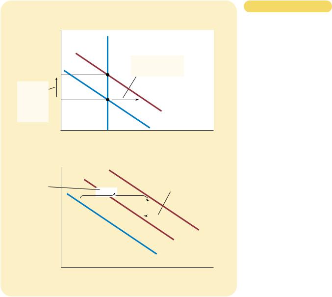
Figur e 20-5
THE CROWDING-OUT EFFECT.
Panel (a) shows the money market. When the government increases its purchases of goods and services, the resulting increase in income raises the demand for money from MD1 to MD2, and this causes the equilibrium interest rate to rise from r1 to r2. Panel (b) shows the effects on aggregate demand. The initial impact of the increase in government purchases shifts the aggregate-demand curve from AD1 to AD2. Yet, because the interest rate is the cost of borrowing, the increase in the interest rate tends to reduce
the quantity of goods and services demanded, particularly for investment goods. This crowding out of investment partially offsets the impact of the fiscal expansion on aggregate demand. In the end, the aggregate-demand curve shifts only to AD3.
interest rates make borrowing more costly, which reduces investment spending. This is the crowding-out effect. Depending on the size of the multiplier and crowding-out effects, the shift in aggregate demand could be larger or smaller than the tax change that causes it.
In addition to the multiplier and crowding-out effects, there is another important determinant of the size of the shift in aggregate demand that results from a tax change: households’ perceptions about whether the tax change is permanent or temporary. For example, suppose that the government announces a tax cut of $1,000 per household. In deciding how much of this $1,000 to spend, households must ask themselves how long this extra income will last. If households expect the
462 |
PART EIGHT SHORT-RUN ECONOMIC FLUCTUATIONS |
|
|
|
|
IN THE NEWS
Japan Tries a
Fiscal Stimulus
No other country has ever poured as much money—more than $830 billion the last 12 months alone—into economic revival as has Japan, and much of that money is now sloshing around the country and creating a noticeable impact. Here in this village in central Japan, as in much of the country, construction crews are busy again, small companies are getting loans again, and some people are feeling a tad more confident.
War II.
To the pessimists Japan is like a vehicle being towed away along the road by all that deficit spending; they doubt its engine will start without an overhaul.
Whatever the reasons for the movement, whatever the concerns for the future, though, the passengers throughout Japan seem relieved that at least the vehicle may be going forward again.
SOURCE: The New York Times, March 11, 1999, p. C1.
tax cut to be permanent, they will view it as adding substantially to their financial resources and, therefore, increase their spending by a large amount. In this case, the tax cut will have a large impact on aggregate demand. By contrast, if households expect the tax change to be temporary, they will view it as adding only slightly to their financial resources and, therefore, will increase their spending by only a small amount. In this case, the tax cut will have a small impact on aggregate demand.
An extreme example of a temporary tax cut was the one announced in 1992. In that year, President George Bush faced a lingering recession and an upcoming reelection campaign. He responded to these circumstances by announcing a reduction in the amount of income tax that the federal government was withholding from workers’ paychecks. Because legislated income tax rates did not change, however, every dollar of reduced withholding in 1992 meant an extra dollar of taxes due on April 15, 1993, when income tax returns for 1992 were to be filed. Thus, Bush’s “tax cut” actually represented only a short-term loan from the government. Not surprisingly, the impact of the policy on consumer spending and aggregate demand was relatively small.
QUICK QUIZ: Suppose that the government reduces spending on highway construction by $10 billion. Which way does the aggregate-demand curve shift? Explain why the shift might be larger than $10 billion. Explain why
the shift might be smaller than $10 billion.
CHAPTER 20 THE INFLUENCE OF MONETARY AND FISCAL POLICY ON AGGREGATE DEMAND |
463 |
F Y I
How Fiscal
Policy Might
Affect
Aggregate
Supply
So far our discussion of fiscal policy has stressed how changes in government purchases and changes in taxes influence the quantity of goods and services demanded. Most economists believe that the short-run macroeconomic effects of fiscal policy work primarily through aggregate demand. Yet fiscal policy can potentially also influence the quantity of goods and ser-
vices supplied.
For instance, consider the effects of tax changes on aggregate supply. One of the Ten Principles of Economics in Chapter 1 is that people respond to incentives. When government policymakers cut tax rates, workers get to keep more of each dollar they earn, so they have a greater incentive to work and produce goods and services. If they respond to this incentive, the quantity of goods and services supplied will be greater at each price level, and the
aggregate-supply curve will shift to the right. Some economists, called supply-siders, have argued that the influence of tax cuts on aggregate supply is very large. Indeed, as we discussed in Chapter 8, some supply-siders claim the influence is so large that a cut in tax rates will actually increase tax revenue by increasing worker effort. Most economists, however, believe that the supply-side effects of tax cuts are much smaller.
Like changes in taxes, changes in government purchases can also potentially affect aggregate supply. Suppose, for instance, that the government increases expenditure on a form of government-provided capital, such as roads. Roads are used by private businesses to make deliveries to their customers; an increase in the quantity of roads increases these businesses’ productivity. Hence, when the government spends more on roads, it increases the quantity of goods and services supplied at any given price level and, thus, shifts the aggregate-supply curve to the right. This effect on aggregate supply is probably more important in the long run than in the short run, however, because it would take some time for the government to build the new roads and put them into use.
USING POLICY TO STABILIZE THE ECONOMY
We have seen how monetary and fiscal policy can affect the economy’s aggregate demand for goods and services. These theoretical insights raise some important policy questions: Should policymakers use these instruments to control aggregate demand and stabilize the economy? If so, when? If not, why not?
THE CASE FOR ACTIVE STABILIZATION POLICY
Let’s return to the question that began this chapter: When the president and Congress cut government spending, how should the Federal Reserve respond? As we have seen, government spending is one determinant of the position of the aggregate-demand curve. When the government cuts spending, aggregate demand will fall, which will depress production and employment in the short run. If the Federal Reserve wants to prevent this adverse effect of the fiscal policy, it can act to expand aggregate demand by increasing the money supply. A monetary expansion would reduce interest rates, stimulate investment spending, and expand aggregate demand. If monetary policy responds appropriately, the combined changes in monetary and fiscal policy could leave the aggregate demand for goods and services unaffected.
This analysis is exactly the sort followed by members of the Federal Open Market Committee. They know that monetary policy is an important determinant

464 |
PART EIGHT SHORT-RUN ECONOMIC FLUCTUATIONS |
of aggregate demand. They also know that there are other important determinants as well, including fiscal policy set by the president and Congress. As a result, the Fed’s Open Market Committee watches the debates over fiscal policy with a keen eye.
This response of monetary policy to the change in fiscal policy is an example of a more general phenomenon: the use of policy instruments to stabilize aggregate demand and, as a result, production and employment. Economic stabilization has been an explicit goal of U.S. policy since the Employment Act of 1946. This act states that “it is the continuing policy and responsibility of the federal government to . . . promote full employment and production.” In essence, the government has chosen to hold itself accountable for short-run macroeconomic performance.
The Employment Act has two implications. The first, more modest, implication is that the government should avoid being a cause of economic fluctuations. Thus, most economists advise against large and sudden changes in monetary and fiscal policy, for such changes are likely to cause fluctuations in aggregate demand. Moreover, when large changes do occur, it is important that monetary and fiscal policymakers be aware of and respond to the other’s actions.
The second, more ambitious, implication of the Employment Act is that the government should respond to changes in the private economy in order to stabilize aggregate demand. The act was passed not long after the publication of John Maynard Keynes’s The General Theory of Employment, Interest, and Money. As we discussed in the preceding chapter, The General Theory has been one the most influential books ever written about economics. In it, Keynes emphasized the key role of aggregate demand in explaining short-run economic fluctuations. Keynes claimed that the government should actively stimulate aggregate demand when aggregate demand appeared insufficient to maintain production at its fullemployment level.
Keynes (and his many followers) argued that aggregate demand fluctuates because of largely irrational waves of pessimism and optimism. He used the term “animal spirits” to refer to these arbitrary changes in attitude. When pessimism reigns, households reduce consumption spending, and firms reduce investment spending. The result is reduced aggregate demand, lower production, and higher unemployment. Conversely, when optimism reigns, households and firms increase spending. The result is higher aggregate demand, higher production, and inflationary pressure. Notice that these changes in attitude are, to some extent, selffulfilling.
In principle, the government can adjust its monetary and fiscal policy in response to these waves of optimism and pessimism and, thereby, stabilize the economy. For example, when people are excessively pessimistic, the Fed can expand the money supply to lower interest rates and expand aggregate demand. When they are excessively optimistic, it can contract the money supply to raise interest rates and dampen aggregate demand. Former Fed Chairman William McChesney Martin described this view of monetary policy very simply: “The Federal Reserve’s job is to take away the punch bowl just as the party gets going.”
CASE STUDY KEYNESIANS IN THE WHITE HOUSE
When a reporter asked President John F. Kennedy in 1961 why he advocated a tax cut, Kennedy replied, “To stimulate the economy. Don’t you remember your

CHAPTER 20 THE INFLUENCE OF MONETARY AND FISCAL POLICY ON AGGREGATE DEMAND |
465 |
Economics 101?” Kennedy’s policy was, in fact, based on the analysis of fiscal policy we have developed in this chapter. His goal was to enact a tax cut, which would raise consumer spending, expand aggregate demand, and increase the economy’s production and employment.
In choosing this policy, Kennedy was relying on his team of economic advisers. This team included such prominent economists as James Tobin and Robert Solow, each of whom would later win a Nobel Prize for his contributions to economics. As students in the 1940s, these economists had closely studied John Maynard Keynes’s General Theory, which then was only a few years old. When the Kennedy advisers proposed cutting taxes, they were putting Keynes’s ideas into action.
Although tax changes can have a potent influence on aggregate demand, they have other effects as well. In particular, by changing the incentives that people face, taxes can alter the aggregate supply of goods and services. Part of the Kennedy proposal was an investment tax credit, which gives a tax break to firms that invest in new capital. Higher investment would not only stimulate aggregate demand immediately but would also increase the economy’s productive capacity over time. Thus, the short-run goal of increasing production through higher aggregate demand was coupled with a long-run goal of increasing production through higher aggregate supply. And, indeed, when the tax cut Kennedy proposed was finally enacted in 1964, it helped usher in a period of robust economic growth.
Since the 1964 tax cut, policymakers have from time to time proposed using fiscal policy as a tool for controlling aggregate demand. As we discussed earlier, President Bush attempted to speed recovery from a recession by reducing tax withholding. Similarly, when President Clinton moved into the Oval Office in 1993, one of his first proposals was a “stimulus package” of increased government spending. His announced goal was to help the U.S. economy recover more quickly from the recession it had just experienced. In the end, however, the stimulus package was defeated. Many in Congress (and many economists) considered the Clinton proposal too late to be of much help, for the economy was already recovering as Clinton took office. Moreover, deficit reduction to encourage long-run economic growth was considered a higher priority than a short-run expansion in aggregate demand.
A VISIONARY AND TWO DISCIPLES
JOHN MAYNARD KEYNES |
JOHN F. KENNEDY |
BILL CLINTON |