1gillman_m_an_introduction_to_mathematical_models_in_ecology

22 CHAPTER 2

Fig. 2.1 Illustration of dynamics of ecological and evolutionary variables with time.

Fig. 2.2 Stability and equilibrium illustrated by a ball in a cup. (a) Displacement of ball from (apparent) equilibrium at position 1 to position 2. (b) Release of ball from position 2 (or equivalent position 3). (c) Displacement of ball beyond local stability boundary at A or A′. (d) Unstable equilibrium.

In order to pursue these lines of enquiry we need to understand some key terms: stability, equilibrium and perturbation. A simple physical model will illustrate these terms. Imagine that a ball is placed in a centre of a cup (Fig. 2.2). The ball is at rest but is it stable? We can only know this if we move the ball; that is, we perturb it. Upon release the ball returns to the base of

the cup. Therefore we can say that the ball at the bottom of the cup is at a position of stable equilibrium, defined as the steady state to which the ball will return after perturbation. Stability is related to equilibrium in that it describes the tendency of a population or other system to stay at or move towards or around the equilibrium. However, the stability of this equilibrium depends on the degree of perturbation. If we push the ball beyond the edge of the cup it falls out of the cup and away from the stable local equilibrium (Fig. 2.2c). The equilibrium is therefore locally stable but not globally stable. The same ideas can be applied to ecosystems or components of ecosystems, such as populations of herbivores or decomposers. Thus for a population or ecosystem the equilibrium or steady state can be defined as the state (e.g. density) to which the population or ecosystem returns after perturbation. The stability of the whole ecosystem can be considered with respect to energy flow, nutrient cycling or the interactions between its components. The distinction between local and global properties of stability is also important here. A population may persist under small amounts of perturbation from its equilibrium value but move towards extinction or outbreak conditions under larger perturbations.

There are other properties of the locally stable equilibrium that we might wish to consider, for example, the rate of return of the ball to the equilibrium after perturbation. The local stability in the physical model of Fig. 2.2 also relies on friction slowing the ball down after release (from position 2); otherwise, with the aid of gravity, it would be like a frictionless pendulum switching continuously from position 2 to 3.

Imagine a second physical model in which we balance the ball on the tip of a pin-head (Fig. 2.2d). The ball is at rest but the equilibrium is highly unstable – any very minor perturbation will send the ball off to another place. Such an unrealistic view of stability features in some ecological models, as you will appreciate later.

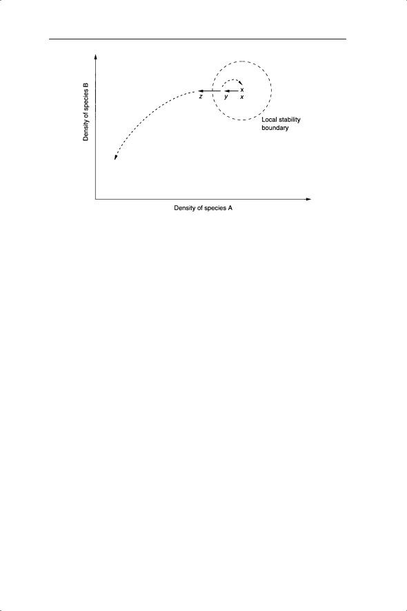
As with the physical model, we can reveal the stability boundaries of the ecological system by perturbation experiments. For example, consider two interacting species such as two competitors or a predator and prey species. Experimental perturbations of the densities of A or B may reveal any stability boundaries (Fig. 2.3). In the example of Fig. 2.3, reduction of the density of species A to value y results in return to the initial (equilibrium) density (x), whereas reduction to z pushes the system beyond the local stability boundary. This could be undertaken in the field as a removal experiment in which the density of species A is reduced by different amounts and its and other (possibly competing) species return to the apparent equilibrium investigated. There are many examples of such experiments involving both removal and addition of species. These studies have been complemented by investigations of the effects of altering abiotic components such as nitrogen levels. Often the results are viewed in terms of the whole community or ecosystem and so a fuller discussion of these studies is reserved for later chapters.

24 CHAPTER 2

Fig. 2.3 Density of species A plotted against the density of species B and illustration of local stability boundaries by displacement from equilibrium (x) to position y or z.

Experimental investigation of stability over an ecologically realistic range of densities will reveal the global stability of the system.

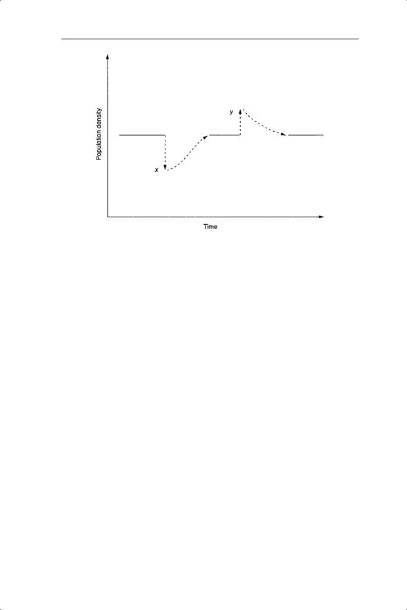
Alternatively, one can look at the dynamics of a population or set of species over time, perturb them to different degrees at certain times and see whether they return to the same (apparent) equilibrium. For example, in Fig. 2.4, increase above or decrease below the steady state reveals the population to be locally stable between the densities x and y. These perturbations are much easier to undertake on a computer than in the field but the possibility does exist for such examinations of stability. Indeed, they may occur as a result of natural perturbations; for example, extreme weather events such as drought or hurricane.

As indicated above, ecosystem stability has been considered, like population stability, as the tendency to move to or return to a stable state. In fact, this embraces two properties of ecosystems: resistance and resilience. Resistance is a measure of the ability of an ecosystem to resist change following a disturbance such as fire or harvesting or following some change in conditions or resource supply. It is usually assessed in terms of the size of the response made to the disturbance or change. Resilience is a measure of the speed with which an ecosystem recovers after a disturbance and returns to a steady state. The effects of fire provide a good illustration of the two terms. Thus northern coniferous forest (taiga) burns easily in summer when conditions are dry, so it has a low resistance to fire. However, because some components such as black spruce (Picea mariana) are adapted to fire (e.g. causing the release of seeds from cones) and because fire releases nutrients from biomass and litter layers, a rapid and predictable secondary succession may

Fig. 2.4 Perturbation of a population away from equilibrium by reduction to density x or increase to density y. In both cases the population returns to the equilibrium, showing it to be locally stable.

follow fire: the system has high resilience after fire. The same arguments can be made for Californian and Mediterranean ecosystems. The idea of resilience was introduced by C.S. Holling in a seminal paper in 1973. Measures of return rates in population studies (Sibly et al. 2007) mirror the ideas of resilience in ecosystems.

2.2 Simple and complex models

Before we begin constructing our first models it is appropriate to pause and think about the rationale of model construction. The complexity of ecology and evolution provide both their fascination and frustration. We are faced with a myriad of species interacting with a variety of abiotic factors, both of which vary in time and space. How then can we begin to model these systems? There are two extremes of approach which have been described by various authors; for example, Maynard Smith’s (1974) distinction between practical ‘simulations’ for particular cases and general ‘models’, May’s (1973a) distinction, following Holling (1966), between detailed ‘tactical’ models and general strategic models and Levins’ (1966) ‘contradictory desiderata of generality, realism and precision’.

At the ‘tactical’ end of the spectrum we attempt to measure all the relevant factors and determine how they interact with the target system, such as a population. For example, in producing a model of change in plant numbers

26 CHAPTER 2

with time we might find that the plants are affected by 12 factors, such as summer rainfall, winter temperatures and levels of herbivory. This information is obtained through field observations and field or laboratory experiments. All the information is combined into a computer program, initial conditions are set (e.g. the number of plants at time 1), values for the different factors entered (e.g. the amount of summer rainfall) and the model run. The output of the model, in this case the number of plants at time t, is then revealed after different periods of time. This is a classic simulation exercise which has become feasible and easy to execute with high computer processing speeds and wide availability of appropriate software.

Now comes the tricky part. We have produced a realistic model in the sense that it mimics closely what we believe is happening in the field. However, we do not really know why it produces a certain answer. The model is intractable (and perhaps unpredictable) owing to its complexity. Tweaking a variable such as rainfall may radically change the output but we may not know why. In other words we have produced a black box which receives a set of variables and generates numbers that vary in time and space. One value of such a model is that it can speed up natural processes so that we do not have to wait 100 years to see how the plant population will (possibly) change, assuming factors remain the same or change in a predictable manner. To get closer to the mechanism(s) in these types of model we have two options. The first is to alter the variables systematically and see how the output responds. This is perhaps best undertaken after the second option, which is to strip the model down to its statistically significant components. You will recall from Chapter 1 that one feature of multiple regression is the removal of non-significant explanatory variables. This will include removing explanatory variables that are correlated. Multiple regression is one example of a set of statistical methods which allow the removal of non-significant terms, resulting in the simplest realistic model (often referred to as the minimal adequate model, especially in connection with particular statistical applications). These methods are consistent with the guiding principle of parsimony which states that the simplest explanation is the best one (Occam’s razor). This principle is relevant to all branches of science. The identification of a common third and hidden variable in the power functions in Chapter 1 follows the principle of parsimony as it replaces two variables by one. In evolutionary biology parsimony has been of fundamental importance in the construction of phylogenetic trees.

From the ‘strategic’ end of the spectrum we can create a model which is so simple that it is known to be unrealistic. What is the value in such an approach? Here the objective is rather different to the simplest realistic model generated from the tactical end. We are using mathematical modelling as a way of formalizing generalizations about the study system. The model is not derived out of consideration of one particular example. It can be argued that strategic models are the most important types of model as they lie at the core

of realistic models. If we do not understand the mode of operation of strategic models then we can never understand why the particular realistic models do what they do. From a mathematical perspective, strategic models are often designed so that their properties can be revealed through analytical solutions of the underlying equations. For example, the stability boundaries of some simple mathematical models can be determined by manipulation of the equations whereas more complex models cannot be solved in this manner. Examples of these types of solution will be given later in the book.

In the light of this discussion we will begin by exploring the properties of some simple strategic models. In fact the following could be argued as strategic models arising from realistic considerations, encompassing the best of the strategic and tactical approaches.

2.3 Density-independent population dynamics

A species with population dynamics that are relatively easy to model is one that reproduces and then dies in the same year. Certain insect species and annual plants fall into this category.

Consider populations of a hypothetical annual plant. The seed germinates in spring, the seedlings grow in the summer and reach a size for flowering and seed set in late summer. The seed are produced and over-winter in the soil. The life cycle is then repeated (Fig. 2.5). There are many variations on this theme but this is a good starting point. We will assume that the population is closed, meaning that there is no immigration or emigration.

10 at start of year 1,

20 at start of year 2

Germinating seed

Fig. 2.5 Life cycle of an annual plant, showing change from germinating seed in spring of year t, through flowering and seed production in the same year. The survival and fecundity values associated with changes from one stage to the next are shown next to the arrows. The italicized values are an example of the change in numbers, starting with 10 germinating seeds.

28 CHAPTER 2

To model the temporal dynamics of populations of this annual plant we need to estimate survival and fecundity values at different stages in the life cycle (Fig. 2.5). Assume we start with 10 seeds germinating in spring. Of these, just two survive to flower and set seed. Therefore the fraction of germinating seed surviving to flowering plant and seed set is 0.2. We will see later that these survival values can be divided further into different ages or stages of the plant (or other study organism). The fecundity of the plant is given by the average number of seeds per plant. We will take this to be 100. To take us round the life cycle to the germinating seed we now need to know the fraction of seed surviving over winter. This will be taken as 0.1. An equation can now be written for the number of germinating seed next year as a function of numbers this year:

Number of germinating seed next year = number of seed germinating this year × fraction surviving to seed set (0.2) × average number of seeds produced (100) × fraction surviving over winter (0.1)

If number of seed germinating this year is replaced by Nt (number at time t) and number of seed germinating next year is replaced by Nt+1 (number at time t + 1) then we can replace the above expression with a simple algebraic expression. Note that we are assuming that the survival and fecundity rates are constant between years, which allow them to be combined as one parameter:

The two survival fractions combine to give an overall value of fraction of germinating seed surviving to the equivalent point after one generation (in this case the value is 0.02). We could have done the same thing starting at a different point in the life cycle. This overall survival is then multiplied by the fecundity to give an overall measure of the change in numbers from one generation to the next. In this example the value is 2, so that the population doubles in size each year.

In mathematical models of temporal change there are two ways of representing time, which have important implications for the methods used in the modelling and the outputs of the models. In the first case, time may be considered as continuous, so that, in theory, it can be divided up into smaller and smaller units. In the second case, time is considered to be discrete in units of, for example, years. The first case is appropriate to populations of individuals with asynchronous and continuous reproduction such as human populations, whereas the second is appropriate to populations with seasonal or otherwise synchronized reproduction. The population of annual plants treated here fall into the discrete time category. The subscripts t and t + 1 show that we are dealing with a discrete time process, with units of years,

due to the fact that reproduction is annual. Such processes are modelled with difference equations (also known as recurrence equations) which relate events at one time point to those of previous time (variable) points. Equation 2.1 is an example of a difference equation. Difference equations could also be used to link different points in space. Continuous processes are modelled with differential equations. The hypothetical extremes of discrete and continuous time are not always encountered or obvious in the field. Most environments have some form of seasonality, even in tropical habitats. Within the breeding season, there may be one reproduction period or there may be several, possibly overlapping, periods of reproduction. In the latter example a combination of difference and differential equations may be required.

The model in equation 2.1 can be represented as a general algebraic equation (see equation 2.2, below), by letting λ equal the average overall survival value multiplied by the fecundity. λ is known as the finite rate of population change. This value was referred to by May (1981) as the ‘multiplicative growth factor per generation’. We will see later an equivalent term representing the change in numbers of species or other taxonomic unit during evolution. In the example in equation 2.2, λ is equivalent to the number of germinating seed produced in year t + 1 for every germinating seed in year t (Nt+1 divided by Nt). λ could also give a measure of the number of flowering plants in year t + 1 relative to the number in year t. Thus, in different versions of equation 2.2, λ can be used (and will take the same value) for any stage of the life cycle as long as it is expressed relative to the same stage in the previous cycle and the survival and fecundity values remain constant. Numbers of seeds or other stages are often represented as densities; for example, numbers per unit area.

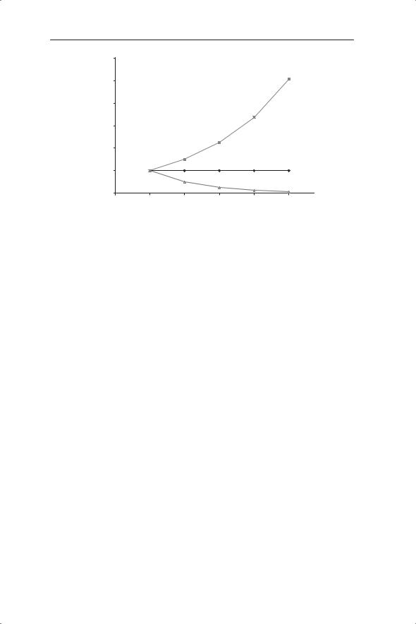
If the survival and fecundity values remain constant the population will change by a multiple of λ every year. The population will increase if λ > 1 and decrease if λ < 1 (Fig. 2.6). At values of λ > 1 we see that increase is geometric or exponential (as expected because the values at time t are multiplied by a fixed amount). Note the similarity of the output in equation 2.2 to the exponential functions shown in Chapter 1 (Fig. 1.10). Equation 2.2 is an example of a density-independent model because the value of λ does not change with population density. The Fibonacci model discussed in Chapter 1 is also an example of a density-independent model.

The serious limitation of density-independent dynamics is that they predict an unrealistic world either eventually covered in one species (when λ > 1) or without a given species (when λ < 1). There is also the possibility of no change in population size if the death rates are exactly balanced by the birth rates: λ = 1. This is also unrealistic because birth and death rates have to be exactly matched or balanced by immigration/emigration for an indefinite period of time. This is the model of the ball balanced on the pin-head (Fig.

Million years

−0

−1

−2

Fig. 2.7 Diversification of a clade with dichotomous branching of taxa every million years.

Imagine a clade in the early stages of diversification. For convenience we will assume time units of millions of years (Myr) and that each end point is a species. At time point 1 there are two species in existence (Fig. 2.7). During the next million years (up to 2 Myr after the clade has existed) each of the existing two species splits to form two new species; that is, four in total. If this process continues at the same rate during subsequent million-year periods the numbers will increase geometrically: 2, 4, 8, 16 and so on. This scenario does not assume any extinction events. We can model extinction in a simple manner by assuming that a certain fraction of taxa go extinct during each time period – for example 0.25 – and therefore 0.75 survive. This model is identical to the density-independent population model (equation 2.2). In this case:

Nt +1 = 2 × 0.75 × Nt

Nt +1 = 1.5Nt

where Nt is the number of species at the end of a given time period. You will see that we also have a parameter equivalent to λ, the finite rate of population increase. This can be defined as a diversification rate, for which we will use the symbol R. In Chapter 3 we will discuss ways in which these processes can be modelled as probabilities (or as values sampled from a probability distribution) rather than fixed values.

In Chapter 1 we saw that equations such as 2.1 and 2.2, in which terms are multiplied, can be log-transformed to produce an additive model. A logtransformation of the diversification equivalent of equations 2.1 or 2.2 yields:

Note that, for a given base, log(ab) = log(a) + log(b). As R represents originations (‘births’, B) of lineages multiplied by the fraction not going extinct (S, surviving) we can write R = BS. Evolutionary biologists are interested in the extinction rate (E) so we can replace S with 1 − E:

R = B(1 − E)