

1gillman_m_an_introduction_to_mathematical_models_in_ecology
.pdf82 CHAPTER 5
Fig. 5.6 Estimated values of λ and b (see text) for 28 populations of insect, overlaid on regions of different dynamic behaviour (open circles are data for laboratory populations, closed circles for field populations; Hassell et al. 1976).
debate on the importance of chaos in ecology rumbled on in the 1990s as new analytical techniques were explored. A study by Ellner and Turchin (1995) using three analyses suggested that Nicholson’s blowflies were on the edge of chaos and no population (either in the laboratory or the field) was chaotic for all analyses. This might suggest that chaos is rare in ecological systems. However, extension to multi-species systems suggests that this is not the case (Chapter 7).
The possible presence of chaos in natural systems cautions us against assuming that all fluctuations are caused by stochastic events. The implication for population regulation is that density dependence is only stabilizing under certain conditions. If density dependence is coupled with high rates of population increase then chaos may result, which destabilizes the population.
We will now consider how to gain an analytical insight into the dynamic behaviour of the discrete logistic. First, the local equilibrium value for stable dynamics can be found. This is achieved by realizing that at equilibrium Nt+1 = Nt; thus there is no change in the population density over time. If we replace Nt+1 by Nt in equation 5.4:
Nt = Nt λ(1 − Nt K ) |
(5.6) |
we can then divide both sides by Nt to give 1 = λ(1 − Nt/K) and rename Nt as N*, defined as the equilibrium value. This equation can be rearranged to make N* the subject of the equation:

REGULATION IN TEMPORAL MODELS |
83 |
1 = λ(1 − N* K ) 1
K ) 1 λ = 1 − N*
 K N*
K N* K = 1 − (1
 λ)
λ)
N* = K(1 − (1 λ)) |
(5.7) |
If we now substitute the values for K (100) and λ (2) we can see that N* = 100(1 − (1/2)) = 50, which agrees with the result obtained in the simulation. The value of λ at which limit cycles begin can now be determined analytically. This is possible because it is known that limit cycles start when the gradient at equilibrium is equal to −1 (May & Oster 1976). For example, with the discrete logistic, we begin by differentiating equation 5.5 with respect to N:
dNt +1 dNt = λ − (2λNt
  K ) dNt +1
 dNt = λ(1 − (2Nt
  K ))
K ))
Set dNt+1/dNt equal to −1:
−1 = λ(1 − (2Nt K )) |
(5.8) |
Now solve this at equilibrium N* by substituting K(1 − (1/λ)) from equation 5.7 for Nt in equation 5.8:
−1 = λ(1 − (2K (1 − (1 λ)) K ))
K ))
Cancel the Ks to give:
−1 = λ − 2λ + 2 −3 = −λ λ = 3
Therefore the single stable equilibrium ends and limit cycles begin at λ = 3, which agrees with the simulations in Fig. 5.4. Note again that the analytical method shows that the carrying capacity, K, is not relevant to the dynamics in this model.
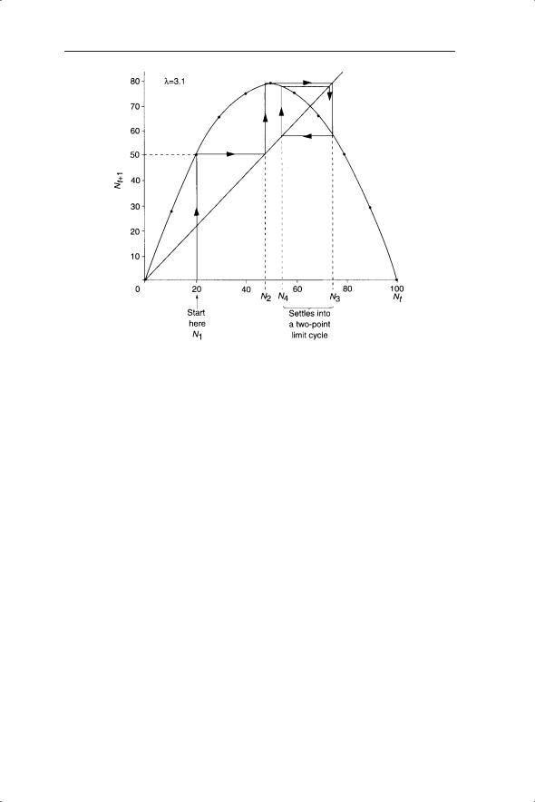
A useful graphical method for analysis of first-order nonlinear difference equations is to plot Nt+1 against Nt (a Ricker–Moran plot; more generally these are known as return maps and can be used with secondand higher-order processes). This was introduced above in the context of distinguishing between random and chaotic dynamics. These plots can be used to iterate the values of the time series as follows. Plot out the curve described by the equation, for example, at λ = 3.1 (Fig. 5.7) and then draw the line of Nt+1 = Nt (the line of unity). The point of intersection of the straight line and the curve tells us the value of N at which the equilibrium occurs. This is a graphical method of solving equation 5.6. To follow the dynamics on a Ricker–Moran
84 CHAPTER 5
Fig. 5.7 Iterations of Nt on a Ricker–Moran plot using the discrete logistic equation with λ = 3.1 and K = 100.
plot we begin at an initial value of Nt, say 20. The next value of N (Nt+1) is read off the curve and, using the line of unity, Nt+1 is changed to Nt and the process repeated. This eventually gives us the two-point limit cycles seen in Fig. 5.4c.
5.5 Re-evaluating the probability of extinction with density dependence
We will now introduce a stochastic element into the discrete logistic model in the same way that we did with the density-independent model (Chapter 3). λ is made to follow the probability density function as in Chapter 3 and the model is run for 20 generations with initial population sizes of one, five and 10. The results of 10 such simulations are illustrated in Table 5.1.
Comparison of the results in Table 5.1 with those in Table 3.1 shows that the probability of extinction has increased and mean persistence time has decreased. Indeed the probability of extinction is the maximum of 1 in each case. At first this seems counter-intuitive, as density dependence has been introduced into the model, which should have a stabilizing influence. However, the high probability of extinction is a result of the assumptions (or model flaw!) inherent in equation 5.4, in particular that at the maximum

REGULATION IN TEMPORAL MODELS |
85 |
Table 5.1 Simulation results for a density-dependent model (equation 5.4) with a probability density function (pdf) for λ as defined in Chapter 3.
Initial population size |
Probability of extinction |
Mean persistence time (generations) |
|
|
|
1 |
1 |
4.3 |
5 |
1 |
6.8 |
10 |
1 |
10.3 |
|
|
|
density of K and above survival is zero. When close to K, the population may still leap above it in one generation, with the result that it becomes extinct in the next generation. So there is now an upper boundary as well as a lower boundary at which the population goes extinct. To remove the upper boundary at K and still retain the density dependence we need to replace the linear density dependence with a nonlinear function.
Instead of the linear density dependence we will use an exponentially declining function (Fig. 5.3) in which the fraction of individuals surviving (s) declines with density (N) according to equation 5.2 (s = e−aN). This leads to a new equation representing the population dynamics of a species with nonlinear density dependence:
Nt +1 = λNt e−aNt |
(5.9) |
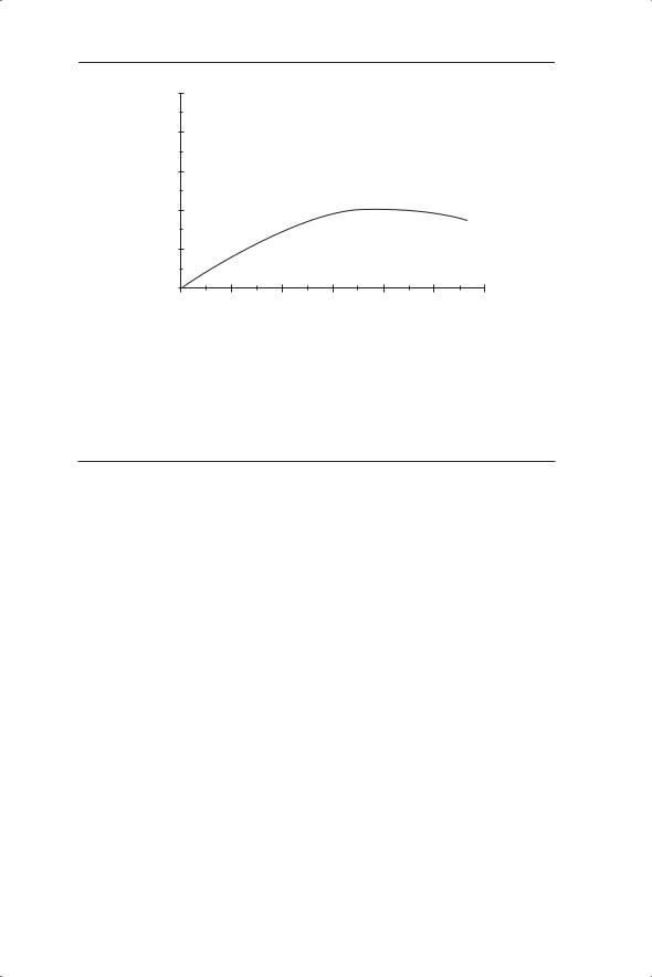
Equation 5.9, like equation 5.4, is a first-order nonlinear difference equation and is known as the Ricker equation (Ricker 1954). This equation has been used extensively in fisheries studies to describe the relationship between recruitment (the number of offspring) and the size of the spawning stock (measured in terms of numbers or biomass). So these examples do not use a full life cycle (Nt+1 as a function of Nt) but instead are considering densitydependent relationships between different stages or ages of a population. We will consider these functions in more detail in Chapter 6 when we discuss the concept of sustainable harvesting (Fig. 5.8 gives an example of a Rickertype curve used to address concerns about a crash in the North Sea cod stocks; Cook et al. 1997).
Once again, simulations to determine the probability of extinction can be generated (Table 5.2) to compare with the two previous models (density-independent and linear density dependence). Both the probabilities of extinction and the mean persistence times are comparable with the densityindependent model (Table 3.1). This is because the model has no upper extinction boundary (unlike the first density-dependent model) but has the same lower extinction boundaries as both previous models. Holmes et al. (2007) describe methods for statistical modelling of population extinction which address issues of density dependence, age structure and species interactions.
86 CHAPTER 5
1,000
|
800 |
recruits |
600 |
of |
|
Number |
400 |
|
|
|
200 |
|
0 |
0
|
|
79 |
|
|
70 |
|
|
|
|
|
|
|
|
|
|
|
76 |
|
|
69 |
|
85 |
83 |
81 |
|
|
|
|
|
|
65 |
|
|
|
93 |
|
78 |
|
66 |
|
|
|
64 |
74 |
|
|||
|
|
77 |
|
|
|
|
|
|
63 |
|
|
72 |
|
91 |
|
|
8082 |
73 |
|
|
88 86 |
|
|
|
|||
94 |
|
|
|
|
||
|
|
|
|
75 |
67 71 |
68 |
90 |
87 |
84 |
|
|
||
92 |
89 |
|
|
|
|
|
50 |
100 |
150 |
200 |
250 |
300 |
|
Spawning stock biomass
Fig. 5.8 Example of a Ricker-type curve used to address concerns about a crash in the North Sea cod stocks (Cook et al. 1997). The fitted curve is in fact a Shepherd stockrecruitment function (R = aS/(1 + (S/b)c)) which produces a similar shape to the Ricker curve but in this case had a slightly better fit (r2 = 0.255, r2 for Ricker curve = 0.234). Numbers indicate years.
Table 5.2 Results from 10 simulations of a density-dependent model (equation 5.9) with a = 0.001 and a pdf for λ as defined in Fig. 3.7.
Initial population size |
Probability of extinction |
Mean persistence time |
|
|
(generations) |
|
|
|
2 |
0.8 |
8.8 |
5 |
0.6 |
12.3 |
10 |
0.4 |
15.9 |
|
|
|
5.6 Estimation of parameters from field data and incorporation of density dependence at different stages in the life cycle
So far we have guessed the parameter values for the density dependence in our model, whereas λ has either been assumed to be constant or drawn from a hypothetical distribution. How can we use field data to estimate the parameter values of the model and therefore make them more realistic? It is possible to set up field or microcosm experiments in which population densities and habitat variables (such as food resources) are manipulated so that densitydependence parameters can be assessed. A second complementary method of estimating density dependence that can also be used to estimate values for λ is to use time-series data; for example, a series of annual censuses, preferably from several sites. Consider the density-dependent model described by the Ricker equation (5.9). A convenient way of estimating the two parameter values (λ and a) is to use linear regression. To start, divide both sides by Nt and take the natural logarithms:
REGULATION IN TEMPORAL MODELS |
87 |
ln (Nt +1 Nt ) = ln (λ) − aNt |
(5.10) |
Now using linear regression of ln(Nt+1/Nt) against Nt we can estimate ln(λ) from the intercept and a from the gradient. With these estimated parameter values we can explore the dynamics of a given population under this model using either simulation or analytical techniques.
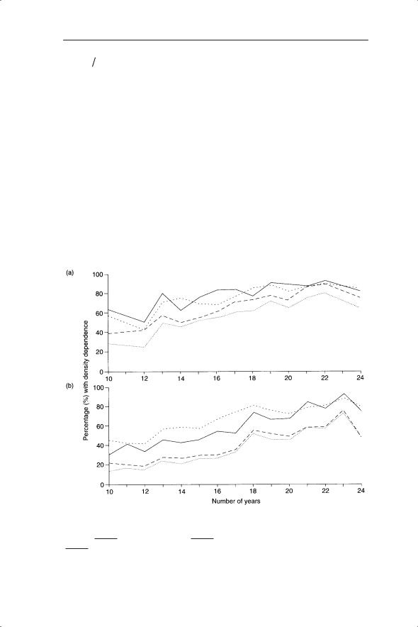
Woiwod and Hanski (1992) used regression of the Ricker equation as one of several measures of density dependence for 94 species of aphid and 263 species of moth collected in the Rothampsted insect survey. This comprehensive analysis showed that detection of density dependence increased with census duration to between 60 and 80% with the Ricker equation being one of two methods to give the highest detection rate (Fig. 5.9).
Although the regression method for detecting density dependence is straightforward we need to be cautious as this method can also detect density dependence from a time series composed of random values. Therefore it may detect density dependence when it is not there (Dennis & Taper 1994, Gillman & Dodd 2000).
Fig. 5.9 Percentage of time series with significant (P < 0.05) density dependence detected
using three methods in (a) aphids and (b) moths. Methods used were Bulmer’s ( |
|
), |
|||
|
|||||
Ricker’s ( |
) and Pollard et al.’s ( |
). The methods are also shown combined |
|
||
( |
). |
|
|
|
|

88 CHAPTER 5
Density dependence may operate at one or more points in the life cycle, which is especially relevant when dealing with species with more complex life cycles. For example, plant species may experience density dependence at the seed, seedling and reproductive stages. Density dependence can operate among seeds if there is a limited number of microsites for germination and only one seed can germinate per microsite. If this is the case, as the density of seeds increases there will be a decreasing fraction that can germinate. Similarly, at the other end of the life cycle, if plants are insect pollinated and there is a fixed number of pollinators, higher densities of flowers may result in a decreased fraction of insect visits. In this case, there may be the opposite effect of enhanced visits to higher-density clumps, although the overall visitation decline will occur at some point of overall flower density.
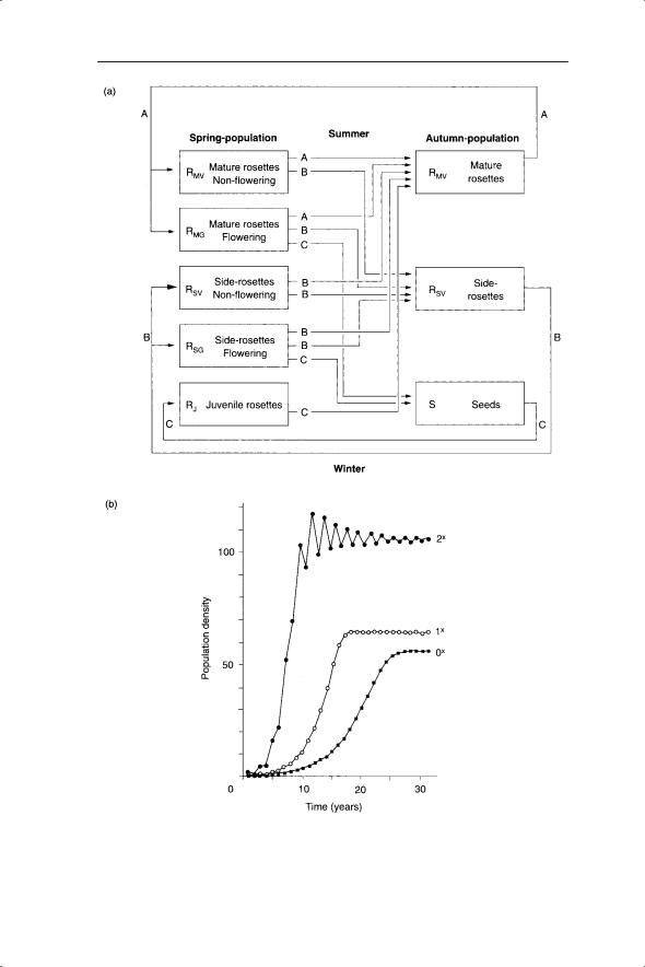
Some studies have actively sought to investigate density dependence at different stages (Gillman et al. 1993). An example of the inclusion of density dependence in a stage-structured model is that of de Kroon et al. (1987). They investigated the effects of mowing as a management regime on the perennial rosette-forming Hypochaeris radicata. Density dependence was incorporated at both germination and seedling establishment, which were in turn functions of gaps in the vegetation. Their stage-structured model had four stages (seeds and three stages of rosette, the latter two of which were further divided into flowering and non-flowering; Fig. 5.10a). The time steps were between seasons rather than years. The authors also argued that a sigmoidal (s-shaped) rather than negative exponential form of density dependence was most appropriate (see Gillman & Crawley 1990 for an example of how tweaking a sigmoidal density-dependent function can lead to the different outcomes of stability, limit cycles and chaos). The results of their model under different mowing frequencies are shown in Fig. 5.10b. Increasing mowing frequency produced more gaps in the vegetation and higher germination, seedling establishment/survival and rosette survival. The net result was that population growth rates were predicted to be higher with increased mowing frequency. The highest mowing frequency produced damped oscillations in the model (Fig. 5.10b).
Given that density dependence can occur at different life-cycle stages and we know that it may cause different dynamical behaviours, it is of interest to know how different types of density dependence may interact. This issue has been explored by Buckley et al. (2001), who contrasted the behaviour of a single difference equation incorporating density dependence (the model of Hassell et al. 1976) and a second model which included a maximum of three density-dependent functions which affected probability of flowering, probability of survival to reproduction and fecundity per flowering plant. Both models performed well as a description of the dynamics while a systematic removal of the components of the second model showed the importance of the strong density dependence in fecundity. Other examples of modelling of annual plants and the importance of factors such as density
REGULATION IN TEMPORAL MODELS |
89 |
Fig. 5.10 (a) Life history of Hypochaeris radicata as used in the model of de Kroon et al. (1987). The three main life-history pathways are survival of adults (A), vegetative propagation (B) and sexual reproduction (C). (b) Simulated population growth of
H. radicata with three mowing frequencies.
90 CHAPTER 5
dependence, spatial dynamics and parameter uncertainty can be found in the review of Holst et al. (2007) and the discussion in Freckleton et al. (2008).
5.7 Density dependence in models of continuous populations
Both Nt+1 = λNt (equation 2.2) and dN/dt = rNt (equation 2.11) are densityindependent equations because the growth parameters λ and r are unaffected by density. We can incorporate the ecological realism of density dependence into differential equations for population change in the same way that we did for the difference equation model in section 5.3 (equation 5.4). As there, the simplest of several possible forms of density dependence is a linear reduction in r with density. This is achieved by multiplying r by (1 − Nt/K):
dN dt = rNt(1 − Nt K ) |
(5.11) |
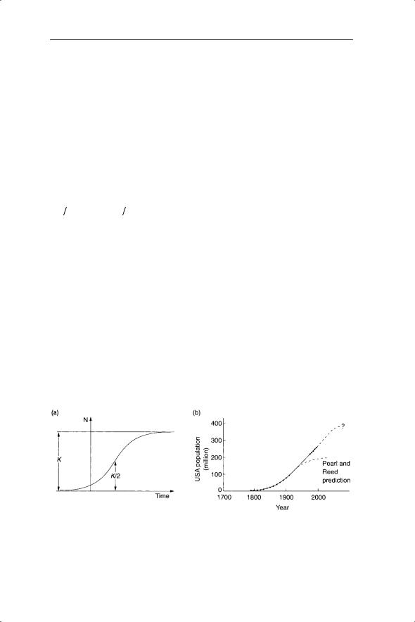
Equation 5.11 is known as the logistic equation, in contrast to its discrete counterpart (equation 5.4). When Nt is close to 0, 1 − Nt/K is close to 1, so the value of r is relatively unaffected. r is steadily reduced as N increases until Nt = K (carrying capacity). At this point there is no change in population size because 1 − Nt/K = 0 and hence dN/dt = 0. If Nt > K then 1 − Nt/K becomes negative, and therefore dN/dt is negative and population size decreases back towards Nt = K. Thus K is a stable equilibrium point. There is a smooth approach to the equilibrium value of K (Fig. 5.11a).
The logistic equation was first used by Verhulst (1838) to describe the growth of human populations and independently by Pearl and Reed (1920) to describe human population growth in the USA (Fig. 5.11b). Hutchinson (1978) and Kingsland (1985) provide fascinating insights into the history of this work. When we first considered the work of Pearl and Reed in Chapter 2 it was to estimate r. It was clear from the residuals of ln (population size) against time that the relationship was nonlinear. Pearl and Reed wanted to
Fig. 5.11 (a) Shape of the logistic curve and relationship to parameters, reprinted from Pearl and Reed (1920). (b) Logistic growth of the human population of the USA from Pearl and Reed (1920) and subsequent data.
REGULATION IN TEMPORAL MODELS |
91 |
ln (population size)
19.8 |
|
|
|
|
|
|
|
19.6 |
|
|
y = 0.0127x Ð 5.9529 |
|
|||
19.4 |
|
|
|
r2 = 0.9942 |
|
|
|
|
|
|
|
|
|
|
|
19.2 |
|
|
|
|
|
|
|
19 |
|
|
|
|
|
1900Ð1999 |
|
18.8 |
|
|
|
|
|
2008 |
|
|
|
|
|
|
Linear (1900Ð1999) |
||
|
|
|
|
|
|
||
18.6 |
|
|
|
|
|
|
|
18.4 |
|
|
|
|
|
|
|
18.2 |
|
|
|
|
|
|
|
18 |
|
|
|
|
|
|
|
1880 |
1900 |
1920 |
1940 |
1960 |
1980 |
2000 |
2020 |
|
|
|
Year |
|
|
|
|
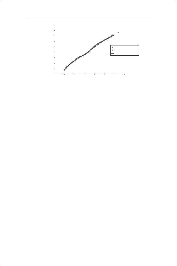
Fig. 5.12 Change in ln (population) size of USA during the twentieth century (www. census.gov/popest/archives/1990s/popclockest.txt).
find a general mathematical description of population growth which starts as exponential growth, but thereafter in their words ‘must develop a point of inflection, and from that point on present a concave face to the x axis and finally become asymptotic, the asymptote representing the maximum number of people which can be supported on the given fixed area’. For this purpose they chose the logistic equation (although in a different form from that discussed here). Pearl and Reed fitted their equation to the population data in Fig. 2.13 to give values of r = 0.0313 and K = 197 000 000. The value of r is close to our linear estimate of 0.027 in Chapter 2. With the benefit of hindsight we know that, in April 2008, the current population of the USA exceeds Pearl and Reed’s estimate of K by about 107 million (www.census.gov/ population/www/popclockus.html). The data set for the twentieth century summarized on the US census website shows an approximately linear increase in ln (population size) with time (Fig. 5.12). There is no evidence yet of an approach towards carrying capacity although there is a suggestion of slowing since about 1990. The linear fit gives a value of r of 0.0127 during the twentieth century.
The lack of agreement between Pearl and Reed’s estimated maximum and the current population size for the USA is due to a variety of causes. For example, the logistic curve is symmetrical so that the population increase before the point of inflexion must equal the population increase after that point (Fig. 5.11a). This may be unrealistic for many population growth curves. Related to this point, Pearl and Reed’s estimates were based on data prior to the point of inflexion. Human carrying capacity is also dependent on changing technology, so that predicted values of carrying capacity based on agricultural productivity and health care in the nineteenth century would inevitably be much lower following the green, biotechnology and medical revolutions of the twentieth century. Pearl and Reed, however, believed that