Econometrics2011

Theorem 9.6.1 Asymptotic Distribution of the Quantile Regression Estimator

When the ’th conditional quantile is linear in x

In general, the asymptotic variance depends on the conditional density of the quantile regression error. When the error ei is independent of xi; then f (0 j xi) = f (0) ; the unconditional density of ei at 0, and we have the simpli…cation

V = (1 2 ) E xix0i 1 : f (0)

A recent monograph on the details of quantile regression is Koenker (2005).

9.7Testing for Omitted NonLinearity

If the goal is to estimate the conditional expectation E(yi j xi) ; it is useful to have a general test of the adequacy of the speci…cation.

One simple test for neglected nonlinearity is to add nonlinear functions of the regressors to the

0 b

regression, and test their signi…cance using a Wald test. Thus, if the model yi = xi + e^i has been …t by OLS, let zi = h(xi) denote functions of xi which are not linear functions of xi (perhaps squares of non-binary regressors) and then …t yi = x0i +z0i~+e~i by OLS, and form a Wald statistic

e

for = 0:

Another popular approach is the RESET test proposed by Ramsey (1969). The null model is

be an (m 1)-vector of powers of y^i: Then run the auxiliary regression

d 2

show that under the null hypothesis, Wn ! m 1: Thus the null is rejected at the % level if Wn exceeds the upper % tail critical value of the 2m 1 distribution.

To implement the test, m must be selected in advance. Typically, small values such as m = 2, 3, or 4 seem to work best.

The RESET test appears to work well as a test of functional form against a wide range of smooth alternatives. It is particularly powerful at detecting single-index models of the form

yi = G(x0i ) + ei

where G( ) is a smooth “link”function. To see why this is the case, note that (9.13) may be written

which has essentially approximated G( ) by a m’th order polynomial.

9.8Model Selection

In earlier sections we discussed the costs and bene…ts of inclusion/exclusion of variables. How does a researcher go about selecting an econometric speci…cation, when economic theory does not provide complete guidance? This is the question of model selection. It is important that the model selection question be well-posed. For example, the question: “What is the right model for y?” is not well-posed, because it does not make clear the conditioning set. In contrast, the question, “Which subset of (x1; :::; xK) enters the regression function E(yi j x1i = x1; :::; xKi = xK)?”is well posed.

In many cases the problem of model selection can be reduced to the comparison of two nested models, as the larger problem can be written as a sequence of such comparisons. We thus consider the question of the inclusion of X2 in the linear regression

y = X1 1 + X2 2 + e;

where X1 is n k1 and X2 is n k2: This is equivalent to the comparison of the two models

To …x notation, models 1 and 2 are estimated by OLS, with residual vectors e^1 and e^2; estimated variances ^21 and ^22; etc., respectively. To simplify some of the statistical discussion, we will on

c

can write this as M. There are many possible desirable properties for a model selection procedure. One useful property is consistency, that it selects the true model with probability one if the sample is su¢ ciently large. A model selection procedure is consistent if

in…nite dimensional, it is more appropriate to view model selection as determining the best …nite sample approximation.

A common approach to model selection is to base the decision on a statistical test such as the Wald Wn: The model selection rule is as follows. For some critical level ; let c satisfy

and the question is which subset of the coe¢ cients are non-zero (equivalently, which regressors enter the regression).

There are two leading cases: ordered regressors and unordered. In the ordered case, the models are

MK : 1 =6 0; 2 =6 0; : : : ; K =6 0:

which are nested. The AIC selection criteria estimates the K models by OLS, stores the residual variance ^2 for each model, and then selects the model with the lowest AIC (9.14). Similarly for the BIC, selecting based on (9.16).

In the unordered case, a model consists of any possible subset of the regressors fx1i; :::; xKig; and the AIC or BIC in principle can be implemented by estimating all possible subset models. However, there are 2K such models, which can be a very large number. For example, 210 = 1024; and 220 = 1; 048; 576: In the latter case, a full-blown implementation of the BIC selection criterion would seem computationally prohibitive.

Exercises

Exercise 9.1 The data …le cps78.dat contains 550 observations on 20 variables taken from the May 1978 current population survey. Variables are listed in the …le cps78.pdf. The goal of the exercise is to estimate a model for the log of earnings (variable LNWAGE) as a function of the conditioning variables.

(a)Start by an OLS regression of LNWAGE on the other variables. Report coe¢ cient estimates and standard errors.

(b)Consider augmenting the model by squares and/or cross-products of the conditioning variables. Estimate your selected model and report the results.

(c)Are there any variables which seem to be unimportant as a determinant of wages? You may re-estimate the model without these variables, if desired.

(d)Test whether the error variance is di¤erent for men and women. Interpret.

(e)Test whether the error variance is di¤erent for whites and nonwhites. Interpret.

(f)Construct a model for the conditional variance. Estimate such a model, test for general heteroskedasticity and report the results.

(g)Using this model for the conditional variance, re-estimate the model from part (c) using FGLS. Report the results.

(h)Do the OLS and FGLS estimates di¤er greatly? Note any interesting di¤erences.

(i)Compare the estimated standard errors. Note any interesting di¤erences.

Exercise 9.2 In the homoskedastic regression model y = X + e with E(ei j xi) = 0 and E(e2i j

size n: Let ^2 be the estimate of 2: You wish to forecast an out-of-sample value of yn+1 given

^ ^ 2 that xn+1 = x: Thus the available information is the sample (y; X); the estimates ( ; V ; ^ ), the

residuals e^; and the out-of-sample value of the regressors, xn+1:

(a)Find a point forecast of yn+1:

(b)Find an estimate of the variance of this forecast.

Show that the function g(x) which minimizes the MAE is the conditional median m (x) = med(yi j xi):

Exercise 9.5 De…ne

g(u) = 1 (u < 0)

where 1 ( ) is the indicator function (takes the value 1 if the argument is true, else equals zero). Let satisfy Eg(yi ) = 0: Is a quantile of the distribution of yi?

Exercise 9.6 Verify equation (9.11).

Exercise 9.7 In Exercise 8.4, you estimated a cost function on a cross-section of electric companies. The equation you estimated was

(a)Following Nerlove, add the variable (log Qi)2 to the regression. Do so. Assess the merits of this new speci…cation using (i) a hypothesis test; (ii) AIC criterion; (iii) BIC criterion. Do you agree with this modi…cation?

(b)Now try a non-linear speci…cation. Consider model (9.17) plus the extra term 6zi; where

zi = log Qi (1 + exp ( (log Qi 7))) 1 :

In addition, impose the restriction 3 + 4 + 5 = 1: This model is called a smooth threshold model. For values of log Qi much below 7; the variable log Qi has a regression slope of 2: For values much above 7; the regression slope is 2 + 6; and the model imposes a smooth transition between these regimes. The model is non-linear because of the parameter 7:

The model works best when 7 is selected so that several values (in this example, at least 10 to 15) of log Qi are both below and above 7: Examine the data and pick an appropriate range for 7:

(c)Estimate the model by non-linear least squares. I recommend the concentration method:

Pick 10 (or more or you like) values of 7 in this range. For each value of 7; calculate zi and estimate the model by OLS. Record the sum of squared errors, and …nd the value of 7 for which the sum of squared errors is minimized.

(d)Calculate standard errors for all the parameters ( 1; :::; 7).

Fn (y; x) is called the empirical distribution function (EDF). Fn is a nonparametric estimate of F: Note that while F may be either discrete or continuous, Fn is by construction a step function.

The EDF is a consistent estimator of the CDF. To see this, note that for any (y; x); 1 (yi y) 1 (xi x)

p

is an iid random variable with expectation F (y; x): Thus by the WLLN (Theorem 2.6.1), Fn (y; x) ! F (y; x) : Furthermore, by the CLT (Theorem 2.8.1),

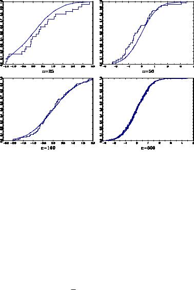
To see the e¤ect of sample size on the EDF, in the Figure below, I have plotted the EDF and true CDF for three random samples of size n = 25; 50, 100, and 500. The random draws are from the N (0; 1) distribution. For n = 25; the EDF is only a crude approximation to the CDF, but the approximation appears to improve for the large n. In general, as the sample size gets larger, the EDF step function gets uniformly close to the true CDF.

Figure 10.1: Empirical Distribution Functions

The EDF is a valid discrete probability distribution which puts probability mass 1=n at each pair (yi; xi), i = 1; :::; n: Notationally, it is helpful to think of a random pair (yi ; xi ) with the

distribution Fn: That is,

Pr(yi y; xi x) = Fn(y; x):

We can easily calculate the moments of functions of (yi ; xi ) :

Z

Eh (yi ; xi ) = h(y; x)dFn(y; x)

Xn

=h (yi; xi) Pr (yi = yi; xi = xi)

i=1

1Xn

=n i=1 h (yi; xi) ;

the empirical sample average.

^

A bootstrap standard error for is the square root of the bootstrap estimate of variance, q

^ ^

s ( ) = Vn :

While this standard error may be calculated and reported, it is not clear if it is useful. The primary use of asymptotic standard errors is to construct asymptotic con…dence intervals, which are based on the asymptotic normal approximation to the t-ratio. However, the use of the bootstrap presumes that such asymptotic approximations might be poor, in which case the normal approximation is suspected. It appears superior to calculate bootstrap con…dence intervals, and we turn to this next.

10.5Percentile Intervals

For a distribution function Gn(u; F ); let qn( ; F ) denote its quantile function. This is the function which solves

Gn(qn( ; F ); F ) = :

[When Gn(u; F ) is discrete, qn( ; F ) may be non-unique, but we will ignore such complications.] Let qn( ) denote the quantile function of the true sampling distribution, and qn( ) = qn( ; Fn) denote the quantile function of the bootstrap distribution. Note that this function will change depending on the underlying statistic Tn whose distribution is Gn:

This is often called the percentile con…dence interval.

Computationally, the quantile qn( ) is estimated by q^n( ); the ’th sample quantile of the simulated statistics fTn1; :::; TnBg; as discussed in the section on Monte Carlo simulation. The