


814 |
CSSE, 2023, vol.47, no.1 |
omegas) to update their positions according to the position of the best search agent. The following formulas are proposed in this regard [14–18]:
→ |
|
= |
|
→ |
→ |
|
|
|
→ |
, |
|
→ |
|
|
→ → |
|
→ |
|
|
|||
Dα |
|
C1.Xα − X |
|
Dβ |
= C2.Xβ − X |
(10) |
||||||||||||||||
→ |
|
|
→ |
→ |
|
|
|
→ |
|
|
|
|
|
|
|
|
|
|
|
|
||
Dδ |
= |
C3.X |
δ |
− |
X |
|
|
|
|
|
|
|
|
|
|
|
|
|||||
|
→ |
|
|
→ |
|
|
→ |
|
|
|
|
|
|
|
|
|||||||
→ |
|
|
|
→ |
. |
|
|
|
, |
|
|
|
→ |
|
→ |
. |
→ |
(11) |
||||
X1 |
|
|
Xα |
|
A1 |
D |
α |
X |
2 |
|
Xβ |
|
A2 |
Dβ |
||||||||
|
|
− |
|
|
|
|
= |
− |
|
|
||||||||||||
|
|
= |
|
|
→ |
|
→ |
|
→ |
|
|
|
|
|||||||||
→ ( |
t + |
1) |
= |
|
X1 |
+ X2 + X3 |
|
|
|
|
|
|
|
(12) |
||||||||
|
|
|
|
|
|
|
|
|
|
|
||||||||||||
X |
|
|
|
|
|
|
|
|
3 |
|
|
|
|
|
|
|
|
|
|
|||
|
|
To mathematically model approaching the prey, we decrease the value of {\displaystyle {\vec {a}}} |
||||||||||||||||||||
→ |
|
|
|
|
|
|
|
|
|
|
|
|
|
|
|
|
|
|
|
|
|
→ |
a. The fluctuation range of {\displaystyle {\vec {A}}} A is also decreased by{\displaystyle {\vec {a}}} |
||||||||||||||||||||||
→ |
|
|
|
|
|
|
|
|
|
|
|
→ |
|
|
|
|
|
|
|
|
|
|
a. In other words, A {\displaystyle {\vec {A}}} is a random value in the interval [−a, a] where a is
→
decreased from 2 to 0 throughout, for iterations. When random values of {\displaystyle {\vec {A}}} A are in [–1, 1], the next position of a search agent can be in any position between its current position and the position of the prey. Gray wolves mostly search according to the position of the alpha, beta,
and delta. They diverge from each other to search for prey and converge to attack prey. {\displaystyle
→
{\vec {A}}} Another component of GWO that favors exploration is {\displaystyle {\vec {C}}} C which contains random values in [0, 2]. This component provides random weights for prey to stochastically
→ |
→ |
emphasize (C > 1) or de-emphasize (C < 1) the effect of prey in defining the distance in Eq. (10).
This assists GWO to show more random behavior throughout optimization, favoring exploration
→
and local optima avoidance. It is worth mentioning here that C is not linearly decreased in contrast
→
to A. For iterations, alpha, beta, and delta wolves estimate the probable position of the prey. Each candidate solution updates its distance from the prey. The parameter a is decreased from 2 to 0 to
emphasize exploration and exploitation, respectively. Candidate solutions tend to diverge from the
→
prey when {\displaystyle |{\vec {A}}| > 1}A > 1 and converge towards the prey when {\displaystyle
→
|{\vec {A}}| < 1}A < 1. Finally, the GWO algorithm is terminated by satisfying an end criterion [19–42].
5 Simulation Results and Analysis
A suitable program for the optimal operation of distributed generation resources and electrical and thermal storage in the microgrid, based on real-time pricing, has been presented. Energy management of resources and electrical and thermal storage was performed using a cost-reduction approach. The GWO algorithm was used for energy management in the microgrid. The algorithm found the optimal variables in such a way that the cost was minimized in the microgrid. The parameters of the proposed GWO are given in Table 1.
Table 1: Parameters of GWO algorithm
Population |
Course of iterations |
σ |
ρ |
ϕ |
100 |
50 |
0.02 |
0.8 |
0.2 |
|
|
|
|
|
CSSE, 2023, vol.47, no.1 |
815 |
Simulations have been performed in two scenarios. In the first one, the energy management was just performed on resources and electrical storage. In contrast, the second scenario, energy management of resources and the combined electrical and thermal storages was simultaneously performed in the microgrid. To verify the results obtained from the simulation, a comparison has been made between the GWO results, and the results obtained from Particle Swarm Optimization (PSO) algorithm, Genetic Algorithm (GA), harmony search (HS), and Artificial Bee Colony (ABC).
5.1 First Scenario
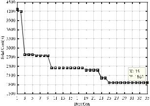
In the first part of the simulations, the energy management of the resources and electrical storage in the microgrid was done by considering the demand response program to reduce the operating cost through the proposed GWO algorithm. Therefore, it was assumed that there was no control over the thermal resources, the required thermal energy of the subscribers was supplied by the boiler without any restrictions, and CHP only produced electrical energy. Also, there was no thermal energy storage in the system. The convergence process of the GWO algorithm in the optimization process is shown in Fig. 5.
Figure 5: Convergence of GWO algorithm in electrical resources management
The energy supply cost without considering the demand response program was $2673, while after optimization through the proposed GWO algorithm, the amount of $1862 was obtained. The GWO algorithm converged to its final value after 25 iterations. In Table 2, the values of the best, the worst, and the average response, as well as the standard deviation for 20 iterations of running the PSO, GA, HS, (ABC) as well as the proposed GWO, are given.
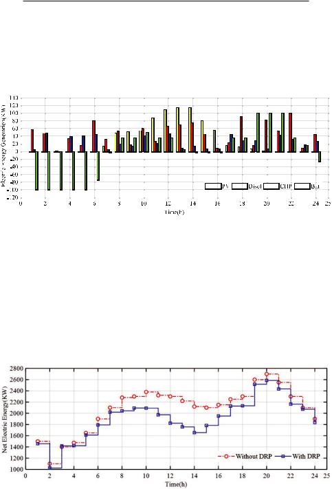
The best responses for the PSO, GA, HS, ABC, and GWO algorithms were obtained as $1908, $1921, $1874, $1893, and $1862, respectively. On the other hand, the low value of standard deviation for the proposed GWO algorithm indicated its higher efficiency, and because if the optimization algorithm has immediate responses to each other in different iterations, then the standard deviation would be at its minimum value. The power generated by the diesel generator, CHP, solar panel, and battery storage in the 24-hour study is shown in Fig. 6 after optimization.
816 CSSE, 2023, vol.47, no.1
Table 2: Optimization results through algorithms in the first scenario
|
Algorithm |
PSO |
GA |
HS |
|
ABC |
GWO |
|
|
|
|
|||||||||||||
|
The best response |
1908 |
1921 |
1874 |
1893 |
|
1862 |
|
|
|
|
|||||||||||||
|
The worst response |
1936 |
1958 |
1891 |
1916 |
|
1873 |
|
|
|
|
|||||||||||||
|
Average |
1919 |
1937 |
1881 |
1903 |
|
1667 |
|
|
|
|
|||||||||||||
|
Standard deviation |
15.4 |
21.8 |
8.3 |
10.1 |
|
6.4 |
|
|
|
|
|
|
|||||||||||
|
|
|
|
|
|
|
|
|
|
|
|
|
|
|
|
|
|
|
|
|
|
|
|
|
|
|
|
|
|
|
|
|
|
|
|
|
|
|
|
|
|
|
|
|
|
|
|
|
|
|
|
|
|
|
|
|
|
|
|
|
|
|
|
|
|
|
|
|
|
|
|
|
|
|
|
|
|
|
|
|
|
|
|
|
|
|
|
|
|
|
|
|
|
|
|
|
|
|
|
|
|
|
|
|
|
|
|
|
|
|
|
|
|
|
|
|
|
|
|
|
|
|
|
|
|
|
|
|
|
|
|
|
|
|
|
|
|
|
|
|
|
|
|
|
|
|
|
|
|
|
|
|
|
|
|
|
|
|
|
|
|
|
|
|
|
|
|
|
|
|
|
|
|
|
|
|
|
|
|
|
|
|
|
|
|
|
|
|
|
|
|
|
|
|
|
|
|
|
|
|
|
|
|
|
|
|
|
|
|
|
|
|
|
|
|
|
|
|
|
|
|
|
|
|
|
|
|
|
|
|
|
|
|
|
|
|
|
|
|
|
|
|
|
|
|
|
|
|
|
|
|
|
|
|
|
|
|
|
|
|
|
|
|
|
|
|
|
|
|
|
|
|
|
|
|
|
|
|
|
|
|
|
|
|
|
|
|
|
|
|
|
|
|
|
|
|
|
|
|
|
|
|
|
|
|
|
|
|
|
|
|
|
|
|
|
|
|
|
|
|
|
|
|
|
|
|
|
|
|
|
|
|
|
|
|
|
|
|
|
|
|
|
|
|
|
|
|
|
|
|
|
|
|
|
|
|
|
|
|
|
|
|
|
|
|
|
|
|
|
|
|
|
|
|
|
|
|
|
|
|
|
|
|
|
|
|
|
|
|
|
|
|
|
|
|
|
|
|
|
|
|
|
|
|
|
|
|
|
|
|
|
|
|
|
|
|
|
|
|
|
|
|
|
|
Figure 6: The transmitted electrical energy with the power grid
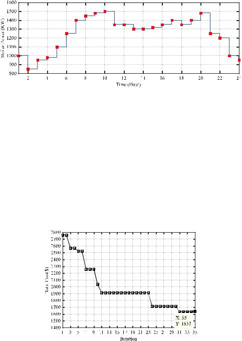
According to Fig. 6, most of the battery storage has been performed from 1:00 a.m. through 6:00 a.m., and most battery discharges occurred from 7:00 p.m. to 9:00 p.m. Batteries play a vital role in supply shifting and reducing costs in demand response programs. The amount of electrical energy transmitted to the nationwide electric network at the time of study is shown in Fig. 7. As illustrated in Fig. 7, the presence of the distributed generation of electrical resources has caused the received electrical energy from the grid to be negative in periods of high demand meaning that the electricity is being sold to the network. Selling electrical energy in periods of high demand, has made a sufficient profit for the microgrid operator, through which the energy supply costs in the microgrid become minimum. For instance, at 10:00 a.m., a profit of about $48.3 was made due to selling electrical energy.
Figure 7: Electrical energy transmitted to the nationwide electric network
CSSE, 2023, vol.47, no.1 |
817 |
The thermal energy produced by the boiler is shown in Fig. 8.
Figure 8: Thermal energy generated by the boiler
It is worth mentioning that, due to a lack of thermal resources management, the produced thermal energy profile by the boiler is precisely similar to the thermal energy needed by the consumers.
5.2 Second Scenario
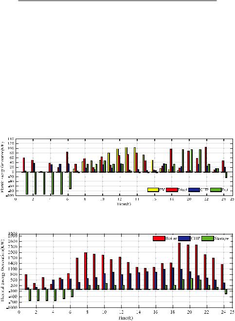
To minimize the energy supply cost in the microgrids, it is required that the demand response program (DRP) be performed considering thermal and electrical resources at the same time because both terms are almost equally effective in the total cost of the microgrid. In the third scenario, thermal and electrical energy management in the microgrid is simultaneously performed using the GWO algorithm. Energy management of diesel generators, solar panels and battery storage as the electrical resources, and boiler with thermal storage has been performed as the thermal distributed generation resources. Finally, CHP has been carried out as the combined heat and power resources in the microgrid. The convergence process of the GWO algorithm in the problem of optimum energy management of thermal and electrical resources in the microgrid is shown in Fig. 9.
Figure 9: Convergence of GWO in thermal and electrical resources management
The cost of the microgrid after optimum management of the combined heat and power through the GWO algorithm was determined as $1637. The GWO algorithm converged to its minimum value
818 |
CSSE, 2023, vol.47, no.1 |
after 31 iterations. Like the two previous scenarios, optimization algorithms were performed for 20 runs, the results of which are given in Table 3.
Table 3: Optimization results by the algorithms in the second scenario
Algorithm |
PSO |
GA |
HS |
ABC |
GWO |
Best response |
1672 |
1684 |
1652 |
1662 |
1637 |
Worst response |
1692 |
1704 |
1667 |
1686 |
1648 |
Average |
1686 |
1692 |
1663 |
1677 |
1642 |
Standard deviation |
15.7 |
19.3 |
8.2 |
9.3 |
6.6 |
|
|
|
|
|
|
The optimization results in the third scenario indicated that the best response in the case of optimization through algorithms of PSO, GA, HS, ABC, and GWO had been calculated as $1672, $1684, $1652, $1662, and $1637, respectively. The slight difference between the obtained responses after 20 iterations of the GWO algorithm led to a standard deviation of 6.6, which is less than the value obtained through other algorithms. In the continuation of the procedure of the performed simulations, the amount of power generated by the electrical resources, and the amount of power generated by the thermal resources during a day in the case of optimization through GWO are shown in Figs. 10 and 11, respectively.
Figure 10: Electrical resource contribution in supplying the required energy
Figure 11: Thermal resource contribution in supplying the required energy in microgrid